As shown earlier, we can create a decision tree using scikit-learn's tree module. For now, let's not specify any optional arguments:

1. We will start off by creating a decision tree:

In [5]: from sklearn import tree
...     dtc = tree.DecisionTreeClassifier()

2. Do you remember how to train the decision tree? We will use the fit function for that:

In [6]: dtc.fit(X_train, y_train)
Out[6]: DecisionTreeClassifier(class_weight=None, criterion='gini',
                               max_depth=None, max_features=None,
                               max_leaf_nodes=None,
                               min_impurity_split=1e-07,
                               min_samples_leaf=1,
                               min_samples_split=2,
                               min_weight_fraction_leaf=0.0,
                               presort=False, random_state=None,
                               splitter='best')

3. Since we did not specify any pre-pruning parameters, we would expect this decision tree to grow quite large and result in a perfect score on the training set:

In [7]: dtc.score(X_train, y_train)
Out[7]: 1.0

However, to our surprise, the test error is not too shabby either:

In [8]: dtc.score(X_test, y_test)
Out[8]: 0.94736842105263153

4. And like earlier, we can find out what the tree looks like using graphviz:

In [9]: with open("tree.dot", 'w') as f:
...         f = tree.export_graphviz(dtc, out_file=f,
...                                  feature_names=data.feature_names,
...                                  class_names=data.target_names)

Indeed, the resulting tree is much more complicated than in our previous example. Don't worry if you are not able to read the content in the diagram. The intent is to see how complex this decision tree is:

At the very top, we find the feature with the name mean concave points to be the most informative, resulting in a split that separates the data into a group of 282 potentially benign samples and a group of 173 potentially malignant samples. We also realize that the tree is rather asymmetric, reaching depth 6 on the left but only depth 2 on the right.

The preceding diagram gives us a good baseline performance. Without doing much, we already achieved 94.7 percent accuracy on the test set, thanks to scikit-learn's excellent default parameter values. But would it be possible to get an even higher score on the test set?

To answer this question, we can do some model exploration. For example, we mentioned earlier that the depth of a tree influences its performance.

5. If we want to study this dependency more systematically, we can repeat building the tree for different values of max_depth:

In [10]: import numpy as np
...      max_depths = np.array([1, 2, 3, 5, 7, 9, 11])

6. For each of these values, we want to run the full model cascade from start to finish. We also want to record the train and test scores. We do this in the for loop:

In [11]: train_score = []
...      test_score = []
...      for d in max_depths:
...          dtc = tree.DecisionTreeClassifier(max_depth=d)
...          dtc.fit(X_train, y_train)
...          train_score.append(dtc.score(X_train, y_train))
...          test_score.append(dtc.score(X_test, y_test))

7. Here, we create a decision tree for every value in max_depths, train the tree on the data, and build lists of all of the train and test scores. We can plot the scores as a function of the tree depth using Matplotlib:

In [12]: import matplotlib.pyplot as plt
...      %matplotlib inline
...      plt.style.use('ggplot')
In [13]: plt.figure(figsize=(10, 6))
...      plt.plot(max_depths, train_score, 'o-', linewidth=3,
...               label='train')
...      plt.plot(max_depths, test_score, 's-', linewidth=3,
...               label='test')
...      plt.xlabel('max_depth')
...      plt.ylabel('score')
...      plt.legend()
Out[13]: <matplotlib.legend.Legend at 0x1c6783d3ef0>

This will produce the following plot:

Now, it becomes evident how the tree depth influences performance. It seems the deeper the tree, the better the performance on the training set. Unfortunately, things seem a little more mixed when it comes to the test set performance. Increasing the depth beyond value 3 does not further improve the test score, so we're still stuck at 94.7 percent. Perhaps there is a different pre-pruning setting we could take advantage of that would work better?

Let's do one more. What about the minimum number of samples required to make a node a leaf node?

8. We repeat the procedure from the previous example:

In [14]: train_score = []
...      test_score = []
...      min_samples = np.array([2, 4, 8, 16, 32])
...      for s in min_samples:
...          dtc = tree.DecisionTreeClassifier(min_samples_leaf=s)
...          dtc.fit(X_train, y_train)
...          train_score.append(dtc.score(X_train, y_train))
...          test_score.append(dtc.score(X_test, y_test))

9. Then, we plot the result:

In [15]: plt.figure(figsize=(10, 6))
...      plt.plot(min_samples, train_score, 'o-', linewidth=3,
...               label='train')
...      plt.plot(min_samples, test_score, 's-', linewidth=3,
...               label='test')
...      plt.xlabel('max_depth')
...      plt.ylabel('score')
....     plt.legend()
Out[15]: <matplotlib.legend.Legend at 0x1c679914fd0>

This leads to a plot that looks quite different from the previous one:

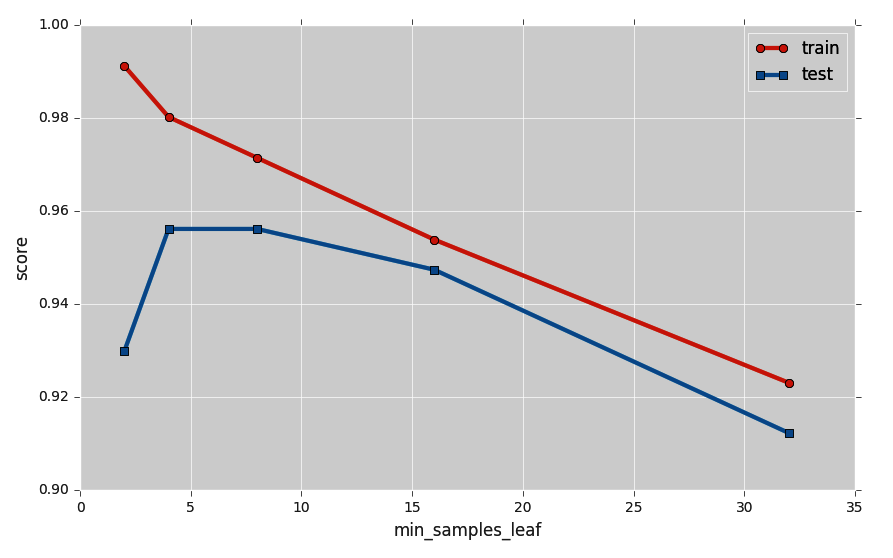
Clearly, increasing min_samples_leaf does not bode well with the training score. But that's not necessarily a bad thing! Because an interesting thing happens in the blue curve: the test score goes through a maximum for values between 4 and 8, leading to the best test score we have found so far—95.6 percent! We just increased our score by 0.9 percent, simply by tweaking the model parameters.

I encourage you to keep tweaking! A lot of great results in machine learning actually come from long-winded hours of trial-and-error model explorations. Before you generate a plot, try thinking about these questions: what would you expect the plot to look like? How should the training score change as you start to restrict the number of leaf nodes (max_leaf_nodes)? What about min_samples_split? Also, how do things change when you switch from the Gini index to information gain?