In the 1950s, American psychologist and artificial intelligence researcher Frank Rosenblatt invented an algorithm that would automatically learn the optimal weight coefficients w₀ and w₁ needed to perform an accurate binary classification: the perceptron learning rule.

Rosenblatt's original perceptron algorithm can be summed up as follows:

1. Initialize the weights to zero or some small random numbers.
2. For each training sample, s_i, perform the following steps:
   1. Compute the predicted target value, ŷ_i.
   2. Compare ŷ_i to the ground truth, y_i, and update the weights accordingly:
      • If the two are the same (correct prediction), skip ahead.
      • If the two are different (wrong prediction), push the weight coefficients, w₀ and w₁, toward the positive or negative target class respectively.

Let's have a closer look at the last step, which is the weight update rule. The goal of the weight coefficients is to take on values that allow for successful classification of the data. Since we initialize the weights either to zero or small random numbers, the chances of getting 100% accuracy from the outset are incredibly low. We therefore need to make small changes to the weights such that our classification accuracy improves.

In the two-input case, this means that we have to update w₀ by some small change Δw₀ and w₁ by some small change, Δw₁:

Rosenblatt reasoned that we should update the weights in a way that makes classification more accurate. We thus need to compare the perceptron's predicted output, ŷ_i, for every data point, i, to the ground truth, y_i. If the two values are the same, the prediction was correct, meaning the perceptron is already doing a great job and we shouldn't be changing anything.

However, if the two values are different, we should push the weights closer to the positive or negative class respectively. This can be summed up with the following equations:

Here, the parameter η denotes the learning rate (usually a constant between 0 and 1). Usually, η is chosen sufficiently small so that with every data sample, s_i, we make only a small step toward the desired solution.

To get a better understanding of this update rule, let's assume that for a particular sample, s_i, we predicted ŷ_i = -1, but the ground truth would have been y_i = +1. If we set η = 1, then we have Δw₀ = (1 - (-1)) x₀ = 2 x₀. In other words, the update rule would want to increase the weight value w₀ by 2 x₀. A stronger weight value would make it more likely for the weighted sum to be above the threshold next time, thus hopefully classifying the sample as ŷ_i = -1 next time around.

On the other hand, if ŷ_i is the same as y_i, then (ŷ_i - y_i) would cancel out, and Δw₀ = 0.

It is straightforward—in a mathematical sense—to extend the perceptron learning rule to more than two inputs, x₀ and x₁, by extending the number of terms in the weighted sum:

It is customary to make one of the weight coefficients not depend on any input features (usually w₀, so x₀ = 1) so that it can act as a scalar (or bias term) in the weighted sum.

To make the perceptron algorithm look more like an artificial neuron, we can illustrate it as follows:

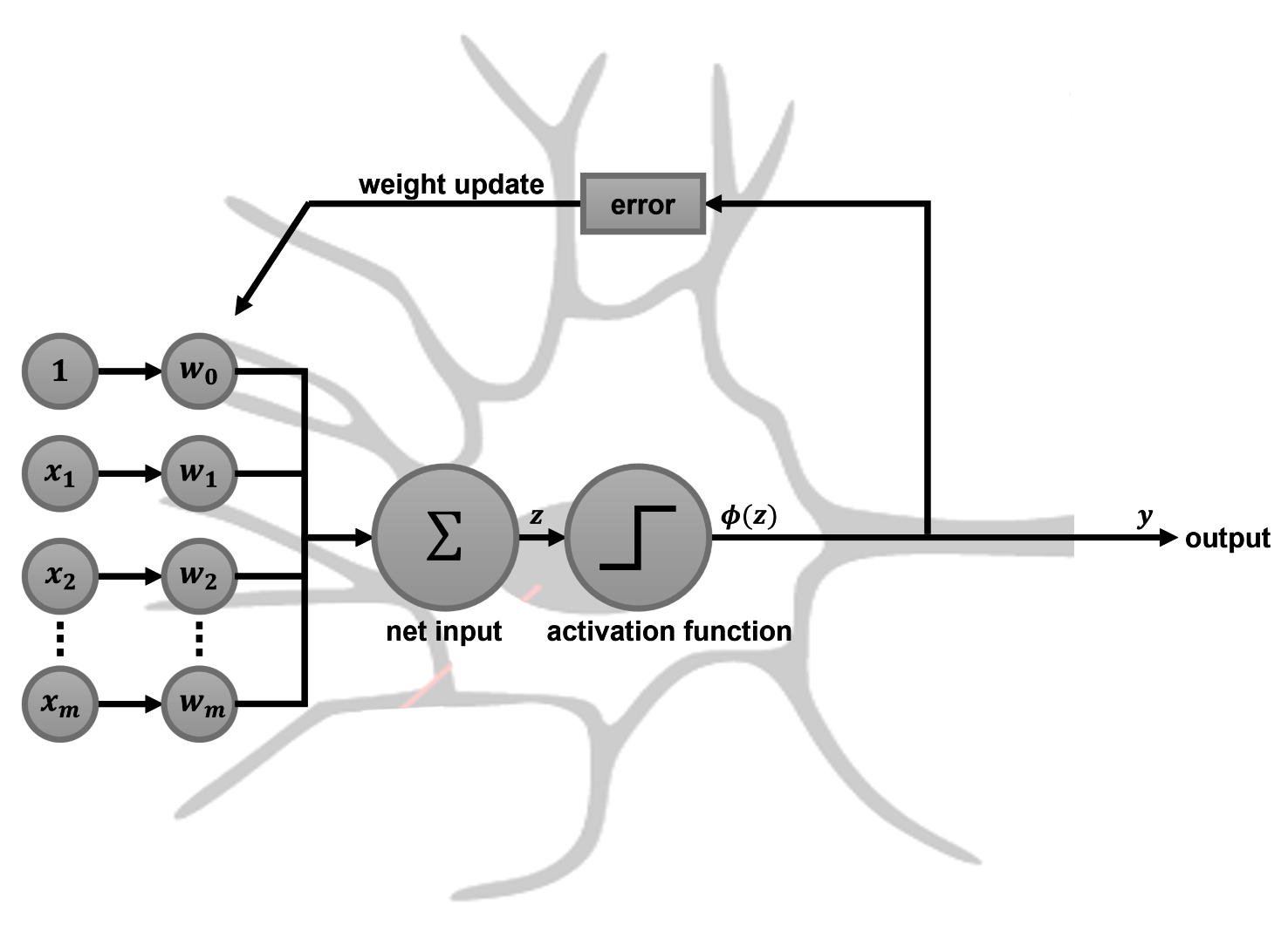
The preceding diagram illustrates the perceptron algorithm as an artificial neuron.

Here, the input features and weight coefficients are interpreted as part of the dendritic tree, where the neuron gets all its inputs from. These inputs are then summed up and passed through the activation function, which happens at the cell body. The output is then sent along the axon to the next cell. In the perceptron learning rule, we also made use of the neuron's output to calculate the error, which, in turn, was used to update the weight coefficients.

Now, let's try it on some sample data!