21

Unemployment

INTRODUCTION

In the real world, full employment is just not possible. All economies experience some unemployment accompanied by low standards of living, hardships, psychological distress and mental agony. Side by side with unemployment, most countries are also plagued with inflation and its related consequences. This chapter deals with inflation and also the relationship between the rate of unemployment and the rate of inflation.

UNEMPLOYMENT AND RELATED TERMS

Unemployed

A person is unemployed if he is out of work and (1) has been actively looking for work during the previous four weeks, or (2) is waiting to be called back to a job after having been laid off.

 

Employed

A person is employed if during the reference week (1) he did any work (at least one hour) as a paid employee, worked in his own business, profession, or on his own farm, or worked 15 hours or more as an unpaid worker in an enterprise operated by a member of a family, or (2) was not working but had a job or business from which he was temporarily absent, whether or not he was paid for the time off or was seeking another job.

Labour Force

Labour force consists of those people who are unemployed as well as those who are employed.

 

Unemployment can be defined more specifically as
Unemployment = Labour Force – Number of people employed

The Unemployment Rate

 

We have,	E =	Total number of employed persons
	U =	Total number of unemployed persons
	L =	Total labour force

 

Using the above notations, we get: L = E = U

Therefore, rate of unemployment

The Unemployment Pool

The unemployment pool consists of the number of unemployed persons at any point of time. As more and more people enter the pool, unemployment increases.

 

There are many reasons why a person may become unemployed. Some of them are as follows:

1. He may be a new entrant or a re-entrant in the labour force.
2. He may have quit the job in order to look for another job and may register as unemployed.
3. He may be laid off.
4. He may lose a job, either by being fired or due to the firm closing down.

Duration of Unemployment

The duration of unemployment is defined as the average length of time for which a person remains unemployed. It indicates whether unemployment is short-term or long-term.

Frequency of Unemployment

The frequency of unemployment is defined as the average number of times, per period, that the workers become unemployed. It depends on two factors:

1. The extent to which demand for labour varies across the different firms in the economy. More the variability, higher is the level of the unemployment rate and vice versa.
2. The growth rate of the labour force. The higher the growth rate, the higher is the rate of unemployment and vice versa.

• The duration of unemployment indicates whether unemployment is short-term or long-term.

TYPES OF UNEMPLOYMENT

Natural Rate of Unemployment

Natural rate of unemployment is the average rate of unemployment around which any economy fluctuates in the long run. Often it is known as NAIRU (Non-accelerating Inflation Rate of Unemployment). It is calculated as:

Natural rate of unemployment for any year

=

Average of unemployment rate for 10 years earlier to ten years later

 

Policies Aimed at Reducing the Natural Unemployment

The government must formulate policies to reduce the natural rate of unemployment. Some policies in this direction are as follows:

1. Unemployment benefits should be reduced as they allow for a longer time period for searching for jobs. These benefits also reduce the urgency for an unemployed person to take up a job.
2. Minimum wages should also be reduced.
3. Incentives should be given to workers to take up technical training. This will make the workers more productive and side by side reduce the natural rate of unemployment.
4. Unemployment hysteresis is a theory, which argues that recessions may permanently affect the natural rate of unemployment. Thus, efforts should be made to control recession.

Frictional Unemployment

Frictional unemployment is the unemployment, which arises due to the time gap it takes for the workers to search for a job that best suits their individual skills and tastes, when the economy is at full-employment. As neither are the workers identical nor are all the jobs identical, it becomes difficult to match the worker’s skills, preferences and their abilities with the job profile. Hence, every economy will have to make do with some extent of frictional unemployment. If frictional unemployment is reduced, then natural rate of unemployment will also fall.

Unemployment in excess of frictional unemployment is what is called cyclical unemployment.

 

Causes of Frictional Unemployment

1. A sectoral shift is actually a change in the composition of demand among the different industries or regions. This occurs due to the advancement of technology and with new inventions. For example, suppose the demand for a good rises due to a fall in its price. This, in turn, leads to a rise in the demand for the labour in this particular industry. Thus, new workers will be attracted to this industry from another industry. This process will take some time. The gap between the time they leave one industry and join another results in frictional unemployment.
2. Workers find themselves out of work unexpectedly due to many reasons; some of them are as follows:
   1. A particular skill in which a worker has expertise may no longer be needed.
   2. A firm may fail and lay off workers.
   3. A worker’s performance may not be satisfactory and thus he is unexpectedly out of work.

Policies Aimed at Reducing Frictional Unemployment

1. The employment agencies of the government can collect information on the workers’ profile and also job profile. Then an effort can be made to match jobs and workers.
2. To make the workers more efficient, retraining programmes can be designed.
3. It is necessary that the terms of the employment insurance programme are not so soft and generous that they encourage the workers to turn down job offers, which they do not find very attractive. Such programmes reduce the uncertainty regarding the workers’ income. However, they raise the level of frictional unemployment.
4. Economists have proposed certain reforms to reduce the level of unemployment; some of them are as follows:
   1. A 100 per cent experience rated system where the firm, which lays off a worker has to bear the entire cost of that worker’s unemployment benefits.
   2. A partially experience rated system where the firm that lays off a worker has to bear a part of the burden of the worker’s unemployment benefits.

Wait Unemployment

Wait unemployment is the unemployment, which is caused by wage rigidity above the equilibrium level which in turn results in job rationing.

 

Job rationing occurs when, at the going wage rate, the supply of labour is greater than the demand for labour. The workers are waiting for jobs to be made available to them. The extent of wait unemployment is shown in Figure 21.1.

Figure 21.1 Wait Unemployment

where,	x-axis = Quantity of Labour
	y-axis = Real Wage

 

OL = Number of labourers who are willing to take up work

SS_L = The supply curve of labour. It is perfectly inelastic at OL units of labour.

DD_L = The demand curve for labour. It is downward sloping.

E^* = Equilibrium takes place at point E^*, where DD_L = SS_L

OW^* = The equilibrium wage rate.

OW₁= Let real wage level be rigid at OW₁. Here the demand for labour is OL₁ and supply of labour is OL. The supply of labour exceeds the demand for labour by L₁L. This excess supply of labour leads to wait unemployment. It is called so as L₁L units of labour are in the market searching and waiting for jobs.

Causes of Wait Unemployment

1. Minimum wage laws aim at protecting and safeguarding the interest of workers against their exploitation by the employers. The minimum wage, or what is also called the floor wage, for certain industries and types of workers, especially the unskilled and inexperienced workers is fixed through legislation, at a level which is above the equilibrium wage rate. The Minimum Wage Law aims at promoting an equitable distribution of income.

   The Minimum Wage Law, however, may add to the already existing level of unemployment. At the high wages, some workers are laid off due to lack of demand. Thus, there is an increase in the unemployment gap.

   An alternative way to increase the income of the poor working class would be, as believed by many economists and policy makers, tax credit. In this scheme, the government makes payment or gives credit to low income families which is more than the tax that they owe to the government.

   BOX 21.3

   Minimum Wage Act was passed in India in 1948 and since then has been revised many times. The Act provides for fixation of minimum wages for notified scheduled employment. As per Government of India, for all the States, the minimum wages have been fixed at about Rs. 40 to 60 per day per person, average about Rs. 50 per day for 25 days per month. It has been successful in raising the level of wages for unskilled and some types of semi-skilled workers, thus improving their productive efficiency.

2. The union is a worker’s organization representing the collective preferences of the members. The union aims at improving the terms of employment, including wages and working conditions, for its members. The union has a strong influence on the social, political and economic life of any economy.

   Often, the union aims at maximizing both employment and wage rate. However, given the downward sloping demand curve of labour, a higher wage rate is possible only with a lower level of employment. Hence, this results in a decrease in employment and an increase in wait unemployment.

3. According to the Efficiency Wage Theory, high wages that are above the level that balances demand and supply often make the workers more efficient. Hence, firms may often give higher wages even at the expense of reducing employment. This again will lead to an increase in wait unemployment.

• Natural unemployment can be reduced through policies aimed at reducing the unemployment benefits and minimum wages and by giving incentives to workers.
• Frictional unemployment can be reduced through collecting information on the workers’ profile to match jobs and workers and through retraining programmes.

COSTS OF UNEMPLOYMENT

The costs of unemployment are as follows:

Loss in Production

It is very obvious that the unemployed do not produce. Thus, there is a lost output which involves a high cost. Arthur Okun has put forward an empirical relationship between unemployment and output. According to Okun’s law, there is a negative relationship between unemployment and the real GDP.

According to this law, 1 extra point of unemployment costs 2 per cent of the GDP.

Okun’s law is depicted in Figure 21.2 as a downward sloping curve showing an inverse relationship between unemployment and the real GDP.

Figure 21.2 Okun’s Law

where,             x-axis = Unemployment rate,

                     y-axis = Real GDP growth rate.

An Undesirable Effect on the Income Distribution and the Human Costs of Unemployment

The costs of recession are borne more by those individuals who have lost their jobs. In the less developed countries, the cost of unemployment is the human misery and poverty which the unemployed have to suffer. In the developed countries, people often have a high standard of living. Recession and the consequential unemployment resulting there from have led to high rates of suicides. Left with no work and thus no sources of income, people are increasingly turning towards crimes.

• According to Okun’s law, there exists a negative relationship between unemployment and the real GDP.
• In the less developed countries, the cost of unemployment is the human misery and poverty which the unemployed have to suffer.

RELATIONSHIP BETWEEN INFLATION AND UNEMPLOYMENT

Phillips’ Curve

The Phillips’ curve is named after the British economist A. W. Phillips who, in the year 1958, presented a study which was based on the behaviour of wages and their relationship to unemployment, in the United Kingdom for the time period 1861 to 1957.

The Phillips’ curve shows that there exists an inverse relationship or trade-off between the rate of unemployment and the rate of increase in money wages or wage inflation. The higher the rate of unemployment, the lower is the rate of wage inflation.

The rate of wage inflation, g_w, can be written as:

 

where,	gw  = the rate of wage inflation
	W   = the wage in the current period
	W–1 = the wage in the preceding period

 

Figure 21.3 Phillips’ Curve for the United Kingdom

The natural rate of unemployment is the amount of frictional unemployment that exists at the level of full employment. We denote it by U^*. The Phillips curve can be presented as:

 

g_w = –e(U – U^*)

where,

 

e	=	It measures the responsiveness of wages to unemployment
U	=	the unemployment rate
U*	=	the natural rate of unemployment
U – U*	=	the unemployment gap

 

From the above equation, the following results emerge:

1. If U > U^*, it implies that the unemployment rate is greater than the natural rate and, hence, the wages fall.
2. If U < U^*, it implies that the unemployment rate is lower than the natural rate and, hence, wages rise.

In Figure 21.3, the original Phillips’ curve has been depicted (for the United Kingdom) as a downward sloping and flat curve showing an inverse relationship between the rate of unemployment and wage inflation.

 

where,	x-axis = unemployment rate
	y-axis = rate of change in money wage rate

 

The original Phillips’ curve shows a negative relationship between the rate of increase in wages and the unemployment rate. Later it came to be described as negative relationship between the rate of increase in prices and the rate of unemployment.

The Phillips’ Curve Relationship: an Explanation

Behaviour of the Organized Labour

An organized labour market can cause autonomous wage increases, which are in excess of the increases in the productivity of labour. This leads to an increase in the prices of goods, resulting in wage-push inflation.

The extent to which the labour market can push through these increases in wages will vary inversely with the unemployment rate in the labour markets:

1. During situations of low unemployment rates and tight labour markets, there is a buoyant demand for goods and the firms are making profits. Under such conditions, an aggressive labour can demand higher wages and the employers often accede to these demands.
2. Alternatively, during situations of high unemployment rates and low profits, the employers resist to even moderate increases in the wages.

Figure 21.4 (a) Labour Market

An Excess Demand for Labour

Figure 21.4 (a) depicts the equilibrium in the labour market.

 

where,	x-axis =	quantity of labour
	y-axis =	wage rate
	SSL     =	the supply curve of labour
	DDL   =	the demand curve for labour
	OW*   =	Equilibrium wage rate where the demand for labour is equal to the supply of labour.
	OW1   =	Wage rate at which there is an excess demand for labour equal to EF.
	OW2   =	Wage rate at which there is an excess demand for labour equal to GH.

 

It is quite obvious that when the wage rate is OW₁, and the excess demand for labour is EF, the increase in wages will be much greater than with the wage rate OW₂ and an excess demand for labour of GH. Thus, the rate of wage increase is inversely related to the amount of excess demand for labour.

This approach can also be expressed in terms of another argument put forward in terms of the Phillips’ curve in Figure 21.4 (b). The amount of unemployment is inversely related to the amount of excess demand for labour.

Figure 21.4 (b) The Phillips’ Curve

Figure 21.4(b) shows

x-axis = unemployment rate

y-axis = rate of change in money wages

OU₁ = Unemployment rate at the equilibrium wage rate OW^* where the demand for labour is equal to the supply of labour. At this level of unemployment, as there is neither excess demand nor excess supply of labour, the rate of wage increase will be zero. At a wage rate lower than OW^*, there will be an excess demand for labour, or in other words, a lower rate of unemployment, and thus a greater increase in the wage rate. This will imply a movement up the Phillips’ curve.

• The explanation of the Phillips’ curve can be expressed in terms of an excess demand for labour and the behaviour of the organized labour which can cause autonomous wage increases.

MODERN PHILLIPS’ CURVE

The original Phillips’ curve was unable to explain the behaviour of unemployment and inflation in the United Kingdom and in the United States after the 1960s. Something was missing from it—the concept of expected inflation. The modern Phillips’ curve or the expectations-augmented Phillips’ curve incorporates the concept of expected inflation.

Milton Friedman and Edmund Phelps have argued that the original Phillips’ curve does not take into consideration the effect of expected inflation in the fixation of the wages. Workers are concerned with their real wages and want that their nominal wages should fully take into consideration the inflation they expect. Thus, workers want to be compensated for expected inflation. Firms, on the other hand, are willing to give higher wages because the goods will be sold in the market at higher prices. Thus, when they are fixing wages and prices, firms and workers take into consideration the expected increase in the price level.

Short-Run Modern Phillips’ Curve

Figure 21.5 depicts the modern Phillips’ curve.

 

where,	x-axis = unemployment rate inflation rate
	y-axis = inflation rate
	U* = natural rate of unemployment

Figure 21.5 Modern Phillips’ Curve: Short-run

PC₁ and PC₂ = These are the short-run modern Phillips’ curves. They are downward sloping and, thus, show a negative relationship between inflation and unemployment in the short-run. The two curves have the same slope showing the same short-run trade-off. However, their height differs because it depends upon the level of expected inflation. The higher the curve higher is the expected inflation for any level of unemployment.

Pont S = It is a point of stagflation. Stagflation is a situation where there is high unemployment and high expected inflation.

 

Long-run Modern Phillips’ Curve

Economists are of the view that the downward sloping Phillips’ curve implying a trade-off between unemployment and inflation is only a short-run phenomenon. The relationship holds only as long as there is a discrepancy between anticipated and actual inflation rate. Once this discrepancy gets removed, the downward sloping Phillips’ curve and the trade-off thereon no longer exist. Thus, in the long run the Phillips’ curve is vertical, implying that the rate of unemployment is independent of the rate of inflation.

Figure 21.6 depicts the vertical or non trade-off Phillips’ curve.

where,

x-axis = unemployment rate

y-axis = inflation rate

PC₁ = initial Phillips’ curve

Point A = Initial point where the rate of unemployment rate is 6 per cent whereas the rate of inflation is 6 per cent.

The government pursues expansionary monetary and fiscal policies, which lead to an increase in aggregate demand. This creates an upward pressure on the rate of inflation, which increases to 8 per cent. The real wage rates experience a decline. This provides an incentive to producers to expand output. This, in turn, leads to an expansion in employment. Over a period of time, the unemployment rate falls and there is a movement upwards along PC₁ to point B.

Point B = The point at which there is an unemployment rate of 4 per cent and inflation rate of 8 per cent. It is reached due to the expansionary monetary and fiscal policies and thus leads to the conventional conclusion of a trade-off between the unemployment rate and inflation rate.

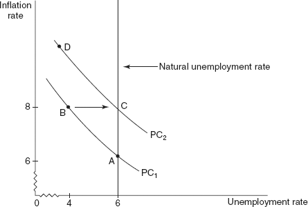
Figure 21.6 Modern Phillips’ Curve: Long Run

However, this trade-off is just a temporary phenomenon. Workers do not take long to realize that inflation has caused a reduction in their real wages. Hence, they demand higher money wages. Once the employers accede to their demands, the real wage rate soon returns to its original level. Due to these adjustments, the Phillips’ curve will shift upward and the unemployment rate will increase and come to its original level of 6 per cent.

PC₂ = The Phillips’ curve after the impact of the monetary and fiscal policies.

Point C = The point at which there is an unemployment rate of 6 per cent and inflation rate of 8 per cent. It is thus showing that the unemployment rate has returned to its original position. Hence, there is now a situation of higher rate of inflation and higher rate of increase in the money wages and an unemployment rate which has not changed from its original 6 per cent rate.

Further expansionary monetary and fiscal policies will lead to movements from C to D, which is quite similar to the movement from A to B. But ultimately the unemployment rate will once again be at 6 per cent while the rate of inflation will rise further.

Thus, the conventional conclusion of a trade-off between the unemployment rate and inflation rate does not hold in the long run. The actual unemployment rate has a tendency to ultimately gravitate towards the equilibrium rate of unemployment, which Friedman calls the natural rate of unemployment, at which the demand for labour is equal to the supply of labour. The long-run Phillips’ curve becomes vertical at 6 per cent, the natural unemployment rate.

Policy Implications of the Phillips’ Curve

Of the many goals that every economic policy aims at achieving, two goals—low inflation and low unemployment—seem to be conflicting. Hence, there is a trade-off between the two goals of low inflation and low unemployment.

According to the Phillips’ curve, policy makers could make a choice between different combinations of the rate of inflation and the rate of unemployment. They could have low inflation but at the cost of high unemployment, or they could maintain low unemployment but only at the cost of a high inflation.

But it has been found that empirical evidence for most of the countries goes against the findings shown by the Phillips’ curve. It seems that even if there is a trade-off, it exists only in the short-run. There is no permanent inflation–unemployment tradeoff, and the policy makers can make a choice between different combinations of unemployment and inflation.

• The short-run modern Phillips’ curve is downward sloping showing a negative relationship between inflation and unemployment in the short-run.
• Stagflation is a situation where there exists high unemployment and high expected inflation.
• In the long-run the Phillips’ curve is vertical, implying that the rate of unemployment is independent of the rate of inflation.
• Empirical evidence for most of the countries goes against the findings shown by the Phillips’ curve. It seems that even if there is a trade-off, it exists only in the short run. There is no permanent inflation–unemployment trade-off, and the policy makers can make a choice between different combinations of unemployment and inflation.

SACRIFICE RATIO

The sacrifice ratio is the percentage of output, which is lost for a one point decrease in the inflation rate. This ratio also depends on the time, place and methods which are used to reduce the inflation. Available estimates show a sacrifice ratio ranging from 1 to 10. Thus in the short-run, the government can reduce inflation but only at the cost of increasing the unemployment and reducing the level of output. Hence, the cost in terms of output of reducing inflation is very high.

 

As already mentioned, the Okun’s law shows that there is a negative relationship between unemployment and the real GDP.

To be more specific, 1 extra point of unemployment costs 2 per cent of GDP.

• Every extra point of unemployment costs 2 per cent of GDP.

INTRODUCTION

In the real world, full employment is just not possible. Side by side with unemployment, most countries are also plagued with inflation.

UNEMPLOYMENT AND RELATED TERMS

Knowledge of the following terms is necessary:

1. Unemployed Person
2. Employed Person
3. Labour Force
4. Unemployment Rate
5. Unemployment Pool
6. Duration of Unemployment
7. Frequency of Unemployment

NATURAL RATE OF UNEMPLOYMENT

1. Natural rate of unemployment is the average rate of unemployment around which any economy fluctuates in the long run.
2. The government must formulate policies to reduce the natural rate of unemployment through:
   1. a reduction in unemployment benefits;
   2. a reduction in the minimum wages;
   3. giving incentives to workers to take up technical training; and
   4. efforts should be made to control recession.

FRICTIONAL UNEMPLOYMENT

1. Frictional unemployment is the unemployment, which arises due to the time gap it takes for the workers to search for a job that best suits their individual skills and tastes, when the economy is at full-employment.
2. The main causes of frictional unemployment are: a change in the composition of demand among the different industries or regions and workers being unexpectedly out of work.
3. Some of the policies for reducing frictional unemployment are:
   1. Collection of information on the workers’ profile and then an effort can be made to match jobs and workers.
   2. Retraining programmes can be designed.

WAIT UNEMPLOYMENT

1. Wait unemployment is the unemployment, which is caused by wage rigidity above the equilibrium level which in turn results in job rationing.
2. The main causes of wait unemployment are:
   1. Minimum wage laws,
   2. The union monopoly power,
   3. Efficiency wages.

COSTS OF UNEMPLOYMENT

The costs of unemployment are: a loss in production as depicted by Okun’s law and an undesirable effect on the distribution of income.

PHILLIPS’ CURVE

1. The Phillips’ curve shows that there exists a trade-off between the rate of unemployment and the rate of increase in money wages or wage inflation.
2. The Phillips’ curve has been depicted as a downward sloping and flat curve showing an inverse relationship between the rate of unemployment and wage inflation.
3. The two explanations for the Phillips’ curve are in terms of
   1. the behaviour of the organized labour, and
   2. an excess demand for labour

MODERN PHILLIPS’ CURVE

The modern Phillips’ curve or the expectations augmented Phillips’ curve incorporates the concept of expected inflation.

SHORT-RUN MODERN PHILLIPS’ CURVE

1. It is downward sloping showing a negative relationship between inflation and unemployment in the short-run.
2. Stagflation is a situation where there is high unemployment and high expected inflation.

LONG-RUN MODERN PHILLIPS’ CURVE

1. The downward sloping Phillips’ curve implying a trade-off between unemployment and inflation is only a short-run phenomenon.
2. In the long-run, the Phillips’ curve is vertical at the natural rate of unemployment, implying that the rate of unemployment is independent of the rate of inflation.
3. The conventional conclusion of a trade-off between the unemployment rate and inflation rate does not hold in the long run.

POLICY IMPLICATIONS OF THE PHILLIPS’ CURVE

1. According to the Phillips’ curve, the two goals of low inflation and low unemployment seem to be conflicting.
2. Empirical evidence shows that there is no permanent inflation-unemployment tradeoff, and the policy makers can make a choice between different combinations of unemployment and inflation.

SACRIFICE RATIO

The sacrifice ratio is the percentage of output, which is lost for a one point decrease in the inflation rate.

TRUE OR FALSE QUESTIONS

1. Labour force consists of only those people who are employed.
2. Natural rate of unemployment is the average rate of unemployment around which any economy fluctuates in the long run.
3. Unemployment in excess of frictional unemployment is called the natural rate of unemployment.
4. Job rationing occurs when, at the going wage rate, the demand for labour is greater than the supply of labour.
5. The Phillips’ curve shows that there exists a direct relationship between the rate of unemployment and the rate of increase in money wages.

VERY SHORT-ANSWER QUESTIONS

1. What is unemployment rate?
2. Write a short note on the unemployment pool.
3. What is the frequency of unemployment?
4. What is the Phillips’ curve? What does it show?
5. What is the modern Phillips’ curve? How is it different from the original Phillips’ curve?

SHORT-ANSWER QUESTIONS

1. Write short notes on
   1. Unemployed
   2. Employed
   3. Labour Force
2. Write short notes on
   1. Wait unemployment
   2. Frictional unemployment
3. The Phillips’ curve shows that there exists a trade-off between the rate of unemployment and the rate of increase in money wages. Explain.
4. What is unemployment? What are the costs of unemployment?
5. Differentiate between frictional unemployment and wait unemployment.

LONG-ANSWER QUESTIONS

1. What is natural rate of unemployment? Suggest some policies to reduce natural rate of unemployment.
2. What is frictional unemployment? What are the causes of frictional unemployment?
3. What is wait unemployment? What are the causes of wait unemployment?
4. Discuss the relationship between Okun’s law and the sacrifice ratio?
5. How do unemployment benefits increase the rate of unemployment? Discuss.

TRUE OR FALSE QUESTIONS

1. False. Labour force consists of those people who are unemployed as well as those who are employed.
2. True. Often it is known as NAIRU, Non-accelerating Inflation Rate of Unemployment.
3. False. Unemployment in excess of frictional unemployment is called cyclical unemployment.
4. False. Job rationing occurs when, at the going wage rate, the supply of labour is greater than the demand for labour. The workers are waiting for jobs to be made available to them.
5. False. The Phillips’ curve shows that there exists an inverse relationship or trade-off between the rate of unemployment and the rate of increase in money wages or wage inflation.