
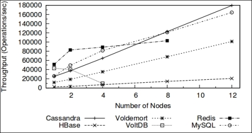
Cassandra is a relative latecomer in the distributed data-store war. It takes advantage of two proven and closely similar data-store mechanisms, namely Bigtable: A Distributed Storage System for Structured Data, 2006 (http://static.googleusercontent.com/external_content/untrusted_dlcp/research.google.com/en//archive/bigtable-osdi06.pdf) and Amazon Dynamo: Amazon's Highly Available Key-value Store, 2007 (http://www.read.seas.harvard.edu/~kohler/class/cs239-w08/decandia07dynamo.pdf). The following diagram displays the read throughputs that show linear scaling of Cassandra:
Like BigTable, it has a tabular data presentation. It is not tabular in the strictest sense. It is rather a dictionary-like structure where each entry holds another sorted dictionary/map. This model is more powerful than the usual key-value store and it is named a table, formerly known as a column family. The properties such as eventual consistency and decentralization are taken from Dynamo.
We'll discuss column family in detail in a later chapter. For now, assume a column family is a giant spreadsheet, such as MS Excel. But unlike spreadsheets, each row is identified by a row key with a number (token), and unlike spreadsheets, each cell may have its own unique name within the row. In Cassandra, the columns in the rows are sorted by this unique column name. Also, since the number of partitions is allowed to be very large (1.7*1038), it distributes the rows almost uniformly across all the available machines by dividing the rows in equal token groups. Tables or column families are contained within a logical container or name space called keyspace. A keyspace can be assumed to be more or less similar to database in RDBMS.
Note
A word on max number of cells, rows, and partitions
A cell in a partition can be assumed as a key-value pair. The maximum number of cells per partition is limited by the Java integer's max value, which is about 2 billion. So, one partition can hold a maximum of 2 billion cells.
A row, in CQL terms, is a bunch of cells with predefined names. When you define a table with a primary key that has just one column, the primary key also serves as the partition key. But when you define a composite primary key, the first column in the definition of the primary key works as the partition key. So, all the rows (bunch of cells) that belong to one partition key go into one partition. This means that every partition can have a maximum of X rows, where X = (2*109/number_of_columns_in_a_row). Essentially, rows * columns cannot exceed 2 billion per partition.
Finally, how many partitions can Cassandra hold for each table or column family? As we know, column families are essentially distributed hashmaps. The keys or row keys or partition keys are generated by taking a consistent hash of the string that you pass. So, the number of partitioned keys is bounded by the number of hashes these functions generate. This means that if you are using the default Murmur3 partitioner (range -263 to +263), the maximum number of partitions that you can have is 1.85*1019. If you use the Random partitioner, the number of partitions that you can have is 1.7*1038.
A Cassandra cluster is called a ring. The terminology is taken from Amazon Dynamo. Cassandra 1.1 and earlier versions used to have a token assigned to each node. Let's call this value the initial token. Each node is responsible for storing all the rows with token values (a token is basically a hash value of a row key) ranging from the previous node's initial token (exclusive) to the node's initial token (inclusive).
This way, the first node, the one with the smallest initial token, will have a range from the token value of the last node (the node with the largest initial token) to the first token value. So, if you jump from node to node, you will make a circle, and this is why a Cassandra cluster is called a ring.
Let's take an example. Assume that there is a hashing algorithm (partitioner) that generates tokens from 0 to 127 and you have four Cassandra machines to create a cluster. To allocate equal load, we need to assign each of the four nodes to bear an equal number of tokens. So, the first machine will be responsible for tokens one to 32, the second will hold 33 to 64, third 65 to 96, and fourth 97 to 127 and 0. If you mark each node with the maximum token number that it can hold, the cluster looks like a ring, as shown in the following figure:
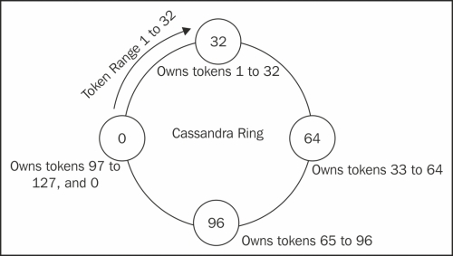
Token ownership and distribution in a balanced Cassandra ring
In Cassandra 1.1 and previous versions, when you create a cluster or add a node, you manually assign its initial token. This is extra work that the database should handle internally. Apart from this, adding and removing nodes requires manual resetting token ownership for some or all nodes. This is called rebalancing. Yet another problem was replacing a node. In the event of replacing a node with a new one, the data (rows that the to-be-replaced node owns) is required to be copied to the new machine from a replica of the old machine (we will see replication later in this chapter). For a large database, this could take a while because we are streaming from one machine. To solve all these problems, Cassandra 1.2 introduced virtual nodes (vnodes).
The following figure shows 16 vnodes distributed over four servers:
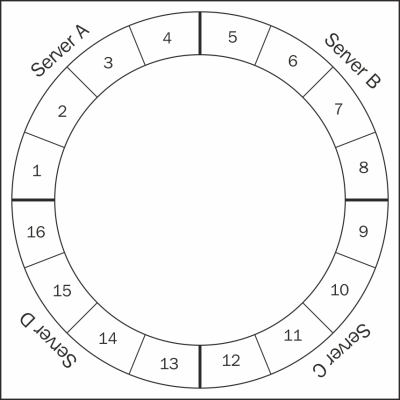
In the preceding figure, each node is responsible for a single continuous range. In the case of a replication factor of 2 or more, the data is also stored on other machines than the one responsible for the range. (Replication factor (RF) represents the number of copies of a table that exist in the system. So, RF=2, means there are two copies of each record for the table.) In this case, one can say one machine, one range. With vnodes, each machine can have multiple smaller ranges and these ranges are automatically assigned by Cassandra. How does this solve those issues? Let's see. If you have a 30 ring cluster and a node with 256 vnodes had to be replaced. If nodes are well-distributed randomly across the cluster, each physical node in remaining 29 nodes will have 8 or 9 vnodes (256/29) that are replicas of vnodes on the dead node. In older versions, with a replication factor of 3, the data had to be streamed from three replicas (10 percent utilization). In the case of vnodes, all the nodes can participate in helping the new node get up.
The other benefit of using vnodes is that you can have a heterogeneous ring where some machines are more powerful than others, and change the vnodes ' settings such that the stronger machines will take proportionally more data than others. This was still possible without vnodes but it needed some tricky calculation and rebalancing. So, let's say you have a cluster of machines with similar hardware specifications and you have decided to add a new server that is twice as powerful as any machine in the cluster. Ideally, you would want it to work twice as harder as any of the old machines. With vnodes, you can achieve this by setting twice as many num_tokens as on the old machine in the new machine's cassandra.yaml file. Now, it will be allotted double the load when compared to the old machines.
Yet another benefit of vnodes is faster repair. Node repair requires the creation of a Merkle tree (we will see this later in this chapter) for each range of data that a node holds. The data gets compared with the data on the replica nodes, and if needed, data re-sync is done. Creation of a Merkle tree involves iterating through all the data in the range followed by streaming it. For a large range, the creation of a Merkle tree can be very time consuming while the data transfer might be much faster. With vnodes, the ranges are smaller, which means faster data validation (by comparing with other nodes). Since the Merkle tree creation process is broken into many smaller steps (as there are many small nodes that exist in a physical node), the data transmission does not have to wait till the whole big range finishes. Also, the validation uses all other machines instead of just a couple of replica nodes.
Tip
As of Cassandra 2.0.9, the default setting for vnodes is "on" with default vnodes per machine as 256. If for some reason you do not want to use vnodes and want to disable this feature, comment out the num_tokens variable and uncomment and set the initial_token variable in cassandra.yaml. If you are starting with a new cluster or migrating an old cluster to the latest version of Cassandra, vnodes are highly recommended.
The number of vnodes that you specify on a Cassandra node represents the number of vnodes on that machine. So, the total vnodes on a cluster is the sum total of all the vnodes across all the nodes. One can always imagine a Cassandra cluster as a ring of lots of vnodes.
Diving into various components of Cassandra without having any context is a frustrating experience. It does not make sense why you are studying SSTable, MemTable, and log structured merge (LSM) trees without being able to see how they fit into the functionality and performance guarantees that Cassandra gives. So first we will see Cassandra's write and read mechanism. It is possible that some of the terms that we encounter during this discussion may not be immediately understandable. The terms are explained in detail later in this chapter.
A rough overview of the Cassandra components is as shown in the following figure:
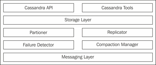
Main components of the Cassandra service
The main class of Storage Layer is StorageProxy. It handles all the requests. The messaging layer is responsible for inter-node communications, such as gossip. Apart from this, process-level structures keep a rough idea about the actual data containers and where they live.
There are four data buckets that you need to know. MemTable is a hash table-like structure that stays in memory. It contains actual cell data. SSTable is the disk version of MemTables. When MemTables are full, they are persisted to hard disk as SSTable. Commit log is an append only log of all the mutations that are sent to the Cassandra cluster.
Commit log lives on the disk and helps to replay uncommitted changes. These three are basically core data. Then there are bloom filters and index. The bloom filter is a probabilistic data structure that lives in the memory. They both live in memory and contain information about the location of data in the SSTable. Each SSTable has one bloom filter and one index associated with it. The bloom filter helps Cassandra to quickly detect which SSTable does not have the requested data, while the index helps to find the exact location of the data in the SSTable file.
With this primer, we can start looking into how write and read works in Cassandra. We will see more explanation later.
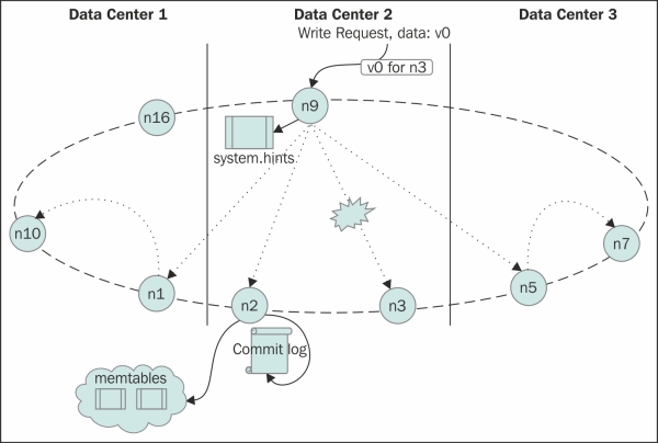
To write, clients need to connect to any of the Cassandra nodes and send a write request. This node is called the
coordinator node. When a node in a Cassandra cluster receives a write request, it delegates the write request to a service called StorageProxy. This node may or may not be the right place to write the data. StorageProxy's job is to get the nodes (all the replicas) that are responsible for holding the data that is going to be written. It utilizes a replication strategy to do this. Once the replica nodes are identified, it sends the RowMutation message to them, the node waits for replies from these nodes, but it does not wait for all the replies to come. It only waits for as many responses as are enough to satisfy the client's minimum number of successful writes defined by ConsistencyLevel.
Note
ConsistencyLevel
is basically a fancy way of saying how reliable a read or write you want to be. Cassandra has tunable consistency, which means you can define how much reliability is wanted. Obviously, everyone wants a hundred percent reliability, but it comes with latency as the cost. For instance, in a thrice-replicated cluster (replication factor = 3), a write time consistency level TWO, means the write will become successful only if it is written to at least two replica nodes. This request will be faster than the one with the consistency level THREE or ALL, but slower than the consistency level ONE or ANY.
The following figure is a simplistic representation of the write mechanism. The operations on node N2 at the bottom represent the node-local activities on receipt of the write request:
The following steps show everything that can happen during a write mechanism:
- If the failure detector detects that there aren't enough live nodes to satisfy
ConsistencyLevel, the request fails. - If the failure detector gives a green signal, but writes time-out after the request is sent due to infrastructure problems or due to extreme load,
StorageProxywrites a local hint to replay when the failed nodes come back to life. This is called hinted hand off.Note
One might think that hinted handoff may be responsible for Cassandra's eventual consistency. But it's not entirely true. If the coordinator node gets shut down or dies due to hardware failure and hints on this machine cannot be forwarded, eventual consistency will not occur. The anti-entropy mechanism is responsible for consistency, rather than hinted hand-off. Anti-entropy makes sure that all replicas are in sync.
- If the replica nodes are distributed across data centers, it will be a bad idea to send individual messages to all the replicas in other data centers. Rather, it sends the message to one replica in each data center with a header, instructing it to forward the request to other replica nodes in that data center.
- Now the data is received by the node which should actually store that data. The data first gets appended to the commit log, and pushed to a MemTable appropriate column family in the memory.
- When the MemTable becomes full, it gets flushed to the disk in a sorted structure named SSTable. With lots of flushes, the disk gets plenty of SSTables. To manage SSTables, a compaction process runs. This process merges data from smaller SSTables to one big sorted file.
Similar to a write case, when StorageProxy of the node that a client is connected to gets the request, it gets a list of nodes containing this key based on the replication strategy. The node's StorageProxy then sorts the nodes based on their proximity to itself. The proximity is determined by the snitch function that is set up for this cluster. Basically, the following types of snitches exist:
SimpleSnitch: A closer node is the one that comes first when moving clockwise in the ring. (A ring is when all the machines in the cluster are placed in a circular fashion with each machine having a token number. When you walk clockwise, the token value increases. At the end, it snaps back to the first node.)PropertyFileSnitch: This snitch allows you to specify how you want your machines' location to be interpreted by Cassandra. You do this by assigning a data center name and rack name for all the machines in the cluster in the$CASSANDRA_HOME/conf/cassandra-topology.propertiesfile. Each node has a copy of this file and you need to alter this file each time you add or remove a node. This is what the file looks like:# Cassandra Node IP=Data Center:Rack 192.168.1.100=DC1:RAC1 192.168.2.200=DC2:RAC2 10.0.0.10=DC1:RAC1 10.0.0.11=DC1:RAC1 10.0.0.12=DC1:RAC2 10.20.114.10=DC2:RAC1 10.20.114.11=DC2:RAC1
GossipingPropertyFileSnitch: ThePropertyFileSnitchis kind of a pain, even when you think about it. Each node has the locations of all nodes manually written and updated every time a new node joins or an old node retires. And then, we need to copy it on all the servers. Wouldn't it be better if we just specify each node's data center and rack on just that one machine, and then have Cassandra somehow collect this information to understand the topology? This is exactly whatGossipingPropertyFileSnitchdoes. Similar toPropertyFileSnitch, you have a file called$CASSANDRA_HOME/conf/cassandra-rackdc.properties, and in this file you specify the data center and the rack name for that machine. The gossip protocol makes sure that this information gets spread to all the nodes in the cluster (and you do not have to edit properties of files on all the nodes when a new node joins or leaves). Here is what acassandra-rackdc.propertiesfile looks like:# indicate the rack and dc for this node dc=DC13 rack=RAC42
RackInferringSnitch: This snitch infers the location of a node based on its IP address. It uses the third octet to infer rack name, and the second octet to assign data center. If you have four nodes10.110.6.30,10.110.6.4,10.110.7.42, and10.111.3.1, this snitch will think the first two live on the same rack as they have the same second octet (110) and the same third octet (6), while the third lives in the same data center but on a different rack as it has the same second octet but the third octet differs. Fourth, however, is assumed to live in a separate data center as it has a different second octet than the three.EC2Snitch: This is meant for Cassandra deployments on Amazon EC2 service. EC2 has regions and within regions, there are availability zones. For example, us-east-1e is an availability zone in the us-east region with availability zone named 1e. This snitch infers the region name (us-east, in this case) as the data center and availability zone (1e) as the rack.EC2MultiRegionSnitch: The multi-region snitch is just an extension ofEC2Snitchwhere data centers and racks are inferred the same way. But you need to make sure thatbroadcast_addressis set to the public IP provided by EC2 and seed nodes must be specified using their public IPs so that inter-data center communication can be done.DynamicSnitch: This Snitch determines closeness based on a recent performance delivered by a node. So, a quick responding node is perceived as being closer than a slower one, irrespective of its location closeness, or closeness in the ring. This is done to avoid overloading a slow performing node.DynamicSnitchis used by all the other snitches by default. You can disable it, but it is not advisable.
Now, with knowledge about snitches, we know the list of the fastest nodes that have the desired row keys, it's time to pull data from them. The coordinator node (the one that the client is connected to) sends a command to the closest node to perform a read (we'll discuss local reads in a minute) and return the data. Now, based on ConsistencyLevel, other nodes will send a command to perform a read operation and send just the digest of the result. If we have read repairs (discussed later) enabled, the remaining replica nodes will be sent a message to compute the digest of the command response.
Let's take an example. Let's say you have five nodes containing a row key K (that is, RF equals five), your read ConsistencyLevel is three; then the closest of the five nodes will be asked for the data and the second and third closest nodes will be asked to return the digest. If there is a difference in the digests, full data is pulled from the conflicting node and the latest of the three will be sent. These replicas will be updated to have the latest data. We still have two nodes left to be queried. If read repairs are not enabled, they will not be touched for this request. Otherwise, these two will be asked to compute the digest. Depending on the read_repair_chance setting, the request to the last two nodes is done in the background, after returning the result. This updates all the nodes with the most recent value, making all replicas consistent.
Let's see what goes on within a node. Take a simple case of a read request looking for a single column within a single row. First, the attempt is made to read from MemTable, which is rapid fast, and since there exists only one copy of data, this is the fastest retrieval. If all required data is not found there, Cassandra looks into SSTable. Now, remember from our earlier discussion that we flush MemTables to disk as SSTables and later when the compaction mechanism wakes up, it merges those SSTables. So, our data can be in multiple SSTables.
The following figure represents a simplified representation of the read mechanism. The bottom of the figure shows processing on the read node. The numbers in circles show the order of the event. BF stands for bloom filter.

Each SSTable is associated with its bloom filter built on the row keys in the SSTable. Bloom filters are kept in the memory and used to detect if an SSTable may contain (false positive) the row data. Now, we have the SSTables that may contain the row key. The SSTables get sorted in reverse chronological order (latest first).
Apart from the bloom filter for row keys, there exists one bloom filter for each row in the SSTable. This secondary bloom filter is created to detect whether the requested column names exist in the SSTable. Now, Cassandra will take SSTables one by one from younger to older, and use the index file to locate the offset for each column value for that row key and the bloom filter associated with the row (built on the column name). On the bloom filter being positive for the requested column, it looks into the SSTable file to read the column value. Note that we may have a column value in other yet-to-be-read SSTables, but that does not matter, because we are reading the most recent SSTables first, and any value that was written earlier to it does not matter. So, the value gets returned as soon as the first column in the most recent SSTable is allocated.
We have gone through how read and write takes place in highly distributed Cassandra clusters. It's time to look into the individual components of it a little deeper.
The messaging service is the mechanism that manages inter-node socket communication in a ring. Communications, for example gossip, read, read digest, write, and so on, processed via a messaging service, can be assumed as a gateway messaging server running at each node.
To communicate, each node creates two socket connections per node. This implies that if you have 101 nodes, there will be 200 open sockets on each node to handle communication with other nodes. The messages contain a verb handler within them that basically tells the receiving node a couple of things: how to deserialize the payload message and what handler to execute for this particular message. The execution is done by the verb handlers (sort of an event handler). The singleton class that orchestrates the messaging service mechanism is org.apache.cassandra.net.MessagingService.
Cassandra uses the gossip protocol for inter-node communication. As the name suggests, the protocol spreads information in the same way an office rumor does. It can also be compared to a virus spread. There is no central broadcaster, but the information (virus) gets transferred to the whole population. It's a way for nodes to build the global map of the system with a small number of local interactions.
Cassandra uses gossip to find out the state and location of other nodes in the ring (cluster). The gossip process runs every second and exchanges information with, at the most, three other nodes in the cluster. Nodes exchange information about themselves and other nodes that they come to know about via some other gossip session. This causes all the nodes to eventually know about all the other nodes. Like everything else in Cassandra, gossip messages have a version number associated with them. So, whenever two nodes gossip, the older information about a node gets overwritten with newer information. Cassandra uses an anti-entropy version of the gossip protocol that utilizes Merkle trees (discussed later) to repair unread data.
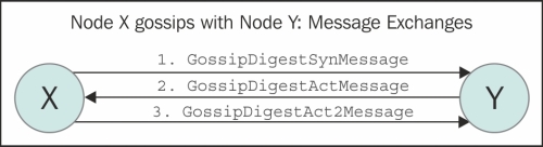
Implementation-wise, the gossip task is handled by the org.apache.cassandra.gms.Gossiper class. The Gossiper class maintains a list of live and dead endpoints (the unreachable endpoints). At each one-second interval, this module starts a gossip round with a randomly chosen node. A full round of gossip consists of three messages. A node X sends a syn message to a node Y to initiate gossip. Y, on receipt of this syn message, sends an ack message back to X. To reply to this ack message, X sends an ack2 message to Y completing a full message round. The following figure shows the two nodes gossiping:
The Gossiper module is linked to failure detection. The module, on hearing one of these messages, updates the failure detector with the liveness information that it has gained. If it hears GossipShutdownMessage, the module marks the remote node as dead in the failure detector.
The node to be gossiped with is chosen based on the following rules:
- Gossip to a random live endpoint
- Gossip to a random unreachable endpoint
- If the node in point 1 was not a seed node or the number of live nodes is less than the number of seeds, gossip to a random seed
Note
Seed node
Seed nodes are the nodes that are first contacted by a newly joining node when they first start up. Seed nodes help the newly started node to discover other nodes in the cluster. It is suggested that to have more than one seed node in a cluster.Seed node is nothing like a master in a master-slave mechanism. It is just another node that helps newly joining nodes to bootstrap gossip protocol. So, seeds are not a
single point of failure (SPOF) and neither has any other purpose that makes them superior.
Failure detection is one of the fundamental features of any robust and distributed system. A good failure detection mechanism implementation makes a fault-tolerant system, such as Cassandra. The failure detector that Cassandra uses is a variation of The ϕ accrual failure detector (2004) by Xavier Défago and others (http://citeseerx.ist.psu.edu/viewdoc/summary?doi=10.1.1.106.3350).
The idea behind a failure detector is to detect a communication failure and take appropriate actions based on the state of the remote node. Unlike traditional failure detectors, phi accrual failure detector does not emit a Boolean alive or dead (true or false, trust or suspect) value. Instead, it gives a continuous value to the application and the application is left to decide the level of severity and act accordingly. This continuous suspect value is called phi (ϕ). So, how does ϕ get calculated?
Let's say we are observing the heartbeat sent from a process on a remote machine. Assume that the latest heartbeat arrived at time Tlast, current time tnow, and Plater(t) is the probability that the heartbeat will arrive t time unit later than the last heartbeat. Then ϕ can be calculated as follows:
ϕ(tnow) = -log10(Plater(tnow – Tlast))
Let's observe this formula informally using common sense. On a sunny day, when everything is fine and the heartbeat is at a constant interval ∆t, the probability of the next heartbeat will keep increasing towards (tnow – Tlast) as one approaches ∆t. So, the value of ϕ will go up. If a heartbeat is not received at ∆t, the more we depart away, the lower the value of Plater becomes, and the value of ϕ keeps on increasing, as shown in the following figure:

In the preceding figure, the curve shows the heartbeat arrival distribution estimate based on past samples. It is used to calculate the value of ϕ based on last arrival, Tlast, and tnow.
One may question as to where a heartbeat is being sent in Cassandra. Gossip has it!
During gossip sessions, each node maintains a list of the arrival time stamps of gossip messages from the other nodes. This list is basically a sliding window, which, in turn, is used to calculate Plater. One may set the sensitivity of the ϕthres threshold.
ϕthres can be understood like this. Let's say we start to suspect whether a node is dead when ϕ >= ϕthres. When ϕthres is 1, it is equivalent to - log(0.1). The probability that we will make a mistake (that is, the decision that the node is dead will be contradicted in future by a late arriving heartbeat) is 0.1 or 10 percent. Similarly, with ϕthres = 2, the probability of making a mistake goes down to 1 percent; with ϕthres = 3, it drops to 0.1 percent; and so on, following log base 10 formula.
Cassandra is a distributed database management system. This means it takes a single logical database and distributes it over one or more machines in the database cluster. So, when you insert some data in Cassandra with a unique row key, based on that row key, Cassandra assigns that row to one of the nodes that's responsible for managing it.
Let's try to understand this. Cassandra inherits a data model from Google's BigTable (http://research.google.com/archive/bigtable.html). This means we can roughly assume that the data is stored in some sort of a table that has an unlimited number of columns (not really unlimited; Cassandra limits the maximum number of cells to be 2 billion per partition) with rows having a unique key, namely row key. Now, your terabytes of data on one machine will be restrictive from multiple points of view. One is disk space, and another is limited parallel processing, and if not duplicated, a source of single point of failure. What Cassandra does is, it defines some rules to slice data across rows and assigns which node in the cluster is responsible for holding which slice. This task is done by a partitioner. There are several types of partitioners to choose from. We'll discuss them in detail in Chapter 4, Deploying a Cluster. In short, Cassandra (as of Version 1.2) offers three partitioners, as follows:
Murmur3Partitioner: This uses a Murmur hash to distribute the data. It performs somewhat better thanRandomPartitioner. It is the default partitioner in Cassandra Version 1.2 onwards.RandomPartitioner: This uses MD5 hashing to distribute data across the cluster. Cassandra 1.1.x and precursors have this as the default partitioner.ByteOrderPartitioner: This keeps keys distributed across the cluster by key bytes. This is an ordered distribution, so the rows are stored in lexical order. This distribution is commonly discouraged because it may cause a hotspot. (A hotspot is a phenomenon where some nodes are heavily under load, (the hotspots), while others are not. Essentially, there is an uneven workload.)
One of the key benefits of partitioning data is that it allows the cluster to grow incrementally. What any partitioning algorithm does is it gives a consistent divisibility of data across all available nodes. The token that a node is assigned to by the partitioner also determines the node's position in the ring. Since the partitioner is a global setting, any node in the cluster can calculate which nodes to look for in a given row key. This ability to calculate data-holding nodes without knowing anything other than the row key, enables any node to calculate what node to forward requests to. This makes the node selection process a single-hop mechanism. The following figure shows a Cassandra ring with an alphabetical partitioner, which shows keys owned by the nodes and data replication:
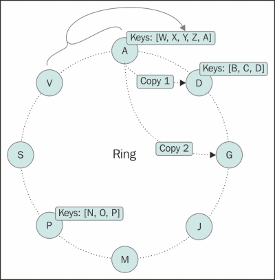
The previous figure shows what an Amazon Dynamo or Cassandra cluster looks like; it looks like a ring. In this particular figure, each node or virtual node is assigned with a letter as its token ID. Let's assume the partitioner in this example slices row keys based on the first letter of the row key (no such default partitioner exists, but you can write one by implementing IPartitioner interface which we will see in Chapter 4, Deploying a Cluster). So, node D will have all the rows whose row keys start with the letters B, C, and D. Since all nodes know about what partitioner and what snitch is being set, they know which nodes have which row keys.
Now that we have observed that partitioning has such a drastic effect on the data movement and distribution, one may think that a bad partitioner can lead to uneven data distribution. In fact, our example ring in the previous paragraph might be a bad partitioner. For a dataset where terms with a specific starting letter have a very high population than the terms with other letters, the ring will be lopsided. A good partitioner is one that is quick to calculate the position from the row key and distributes the row keys evenly; something like a partitioner based on a consistent hashing algorithm.
Cassandra runs on commodity hardware, and works reliably in network partitions. However, this comes with a cost: replication. To avoid data inaccessibility if a node goes down or becomes unavailable, one must replicate data to more than one node. Replication provides features such as fault tolerance and no single point of failure to the system. Cassandra provides more than one strategy to replicate the data, and one can configure the replication factor while creating key space. This will be discussed in detail in Chapter 3, Effective CQL.
Replication is tightly bound to consistency level (CL). CL can be thought of as an answer to the question: How many replicas must respond positively to declare a successful operation? If you have a read consistency level three, that means a client will be returned a successful read as soon as three replicas respond with the data. The same goes for write. For write consistency three, at least three replicas must respond that the write to them was successful. Obviously, the replication factor must be greater than any consistency level, otherwise there will never be enough replicas to write to, or read from, successfully.
Replication should be thought of as an added redundancy. One should never have a replication factor one in their production environment. If you think having multiple writes to different replicas will slow down the writes, you can set up a favorable consistency level. Cassandra offers a set of consistency levels, including fire and forget, CL ZERO, and ensures all replica operations (read and write). This is where the so-called "tunable" consistency of Cassandra lies. The following table shows all the consistency levels:
|
WRITE |
READ | ||
|---|---|---|---|
|
Consistency level |
Meaning |
Consistency level |
Meaning |
|
ZERO |
Fire and forget | ||
|
ANY |
Success on hinted hand off write | ||
|
ONE |
First replica returned successfully |
ONE |
First replica returned successfully |
|
QUORUM |
N/2 + 1 replica success |
QUORUM |
N/2 + 1 replica success |
|
ALL |
All replica success |
ALL |
All replica success |
Imagine that the value of your replication factor is three. This means your data will be stored in three nodes. If you have a write consistency level as one, and a read consistency level as one, they may or may not be consistent. Here is why: when a write happens, the row mutation information is sent to all the nodes, but the user is returned a success message as soon as the first replica responds with a success message. Meanwhile, the data is being written to two other nodes. If a read request comes into those two nodes with a consistency level one, they would return the stale data. Or, if it is a heavy write-read scenario, all the three nodes may have different data at some instant of time, and read with CL=1, which may result in inconsistent reads for a very brief time. The following figure shows reads and writes, on an R + W > N system:
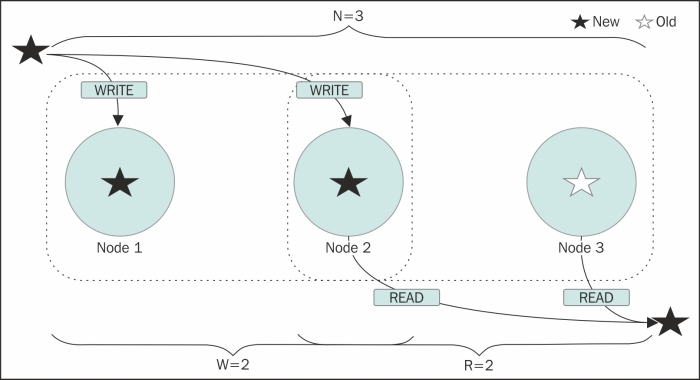
The concept of weak and strong consistencies comes here. Weak consistency is when reads may be wrong for a brief amount of time and strong consistency is when results are always consistent. Basically, weak consistency sometimes returns inconsistent results. If you have an N replica, to ensure that your reads always result in the latest value, you must write and read from as many nodes that ensure at least one node overlaps. So, if you write to W nodes and read from R nodes such that R+W > N, there must be at least one node that is common in both read and write. And this will ensure that you have the latest data. See the previous figure; ZERO and ANY consistency levels are weak consistency. ALL is strong. ONE for read and ALL for write, or vice versa, will make a strongly consistent system.
A system with QUORUM for both, read and write, is a strongly consistent system. Again, the idea is to make sure that between the reads and the writes, at least one node overlaps. While we are on this topic, it may be worth noticing that the higher the consistency level, the slower the operation. So, if you want a super-fast write and a not-so-fast read, and you also want the system to be strongly consistent, you can opt for consistency level ONE for the writes and ALL for the reads.
Cassandra (and HBase) is heavily influenced by LSM tree. It uses an LSM tree-like mechanism to store data on a disk. The writes are sequential (in append fashion) and the data storage is contiguous. This makes writes in Cassandra fast, because there is no disk-seek involved. Contrast this with an RBDMS system that is based on the B+ tree (http://en.wikipedia.org/wiki/B%2B_tree) implementation.
LSM tree advocates the following mechanism to store data: note down the arriving modification into a log file (commit log), push the modification/new data into memory (MemTable) for faster lookup, and when the system has gathered enough updates in memory, or after a certain threshold time, flush this data to a disk in a structured store file (SSTable). The logs corresponding to the updates that are flushed can now be discarded.
LSM trees
Note
For more information, refer to The Log-Structured Merge-Tree (LSM-Tree) (1996) by Patrick O'Neil and others at http://citeseerx.ist.psu.edu/viewdoc/summary?doi=10.1.1.44.2782.
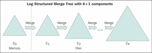
The preceding paper suggests multi-component LSM trees, where data from memory is flushed into a smaller tree on disk for a quicker merge. When this tree fills up, it rolls them into a bigger tree. So, if you have K trees with the first tree being the smallest and the Kth being the largest, the memory gets flushed into the first tree, which when full, performs a rolling merge to the second tree, and so on. The change eventually lands up onto the Kth tree. This is a background process (similar to the compaction process in Cassandra). Cassandra differs a little bit where memory resident data is flushed into immutable SSTables, which are eventually merged into one big SSTable by a background process. Like any other disk-resident access tree, popular pages are buffered into memory for faster access. Cassandra has a similar concept with key cache and row cache (optional) mechanisms.
We'll see the LSM tree in action in the context of Cassandra in the next three sections.
One of the promises that Cassandra makes to the end users is durability. In conventional terms (or in ACID terminology), durability guarantees that a successful transaction (write, update) will survive permanently. This means that once Cassandra says write successful, it means the data is persisted and will survive system failures. This is done the same way as in any DBMS that guarantees durability: by writing the replayable information to a file before responding to a successful write. This log is called the commit log in the Cassandra realm.
This is what happens under the hood: any write to a node gets tracked by org.apache.cassandra.db.commitlog.CommitLog, which writes the data with certain metadata into the commit log file in such a manner that replaying this will recreate the data. The purpose of this exercise is to ensure there is no data loss. If, due to some reason, the data cannot make it into MemTable or SSTable, the system can replay the commit log to recreate the data.
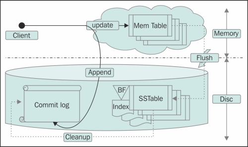
Commit log, MemTable, and SSTable in a node are tightly coupled. Any write operation gets written to the commit log first and then the MemTable gets updated. MemTable, based on certain criteria, gets flushed to a disk in immutable files called SSTable. The data in commit logs gets purged after its corresponding data in MemTable gets flushed to SSTable.
Also, there exists one single commit log per node server. Like any other logging mechanism, the commit log is set to rolling after a certain size. The following figure shows the commit log, MemTable, and SSTable in action:
Let's quickly go a bit deeper into the implementation. All the classes that deal with the commit log management reside under the org.apache.cassandra.db.commitlog package. The commit log singleton is a facade for all the operations. The implementations of ICommitLogExecutorService are responsible for write commands to the commit log file. Then there is a CommitLogSegment class. It manages a single commit log file, writes serialized write (mutation) to the commit log, and it holds a very interesting property: cfLastWrite. The cfLastWrite property is a map with a key as the column family name and value as an integer that represents the position (offset) in the commit log file where the last mutation for that column family is written. It can be thought of as a cursor; one cursor per column family. When the MemTable of a column family is flushed, the segments containing those mutations are marked as clean (for that particular column family). And when a new write arrives, it is marked dirty with offset at the latest mutation.
In events of failure (hardware crash, abrupt shutdown), this is how the commit log helps the system to recover:
- Each commit log segment is iterated in the ascending order of timestamp.
- Lowest
ReplayPosition(which is the offset in commit log that specifies the point till which the data is already stored in SSTables) is chosen from the SSTable metadata. - The log entry is replayed for a column family if the position of the log entry is greater than the replay position in the latest SSTable metadata.
- After the log replay is done, all the MemTables are force flushed to a disk, and all the commit log segments are recycled.
MemTable is an in-memory representation of a column family. It can be thought of as cached data. MemTable is sorted by key. Data in MemTable is sorted by row key. Unlike the commit log, which is append-only, MemTable does not contain duplicates. A new write with a key that already exists in the MemTable, overwrites the older record. This being in memory is both fast and efficient. The following is an example:
Write 1: {k1: [{c1, v1}, {c2, v2}, {c3, v3}]}

In CommitLog (new entry, append):
  {k1: [{c1, v1},{c2, v2}, {c3, v3}]}

In MemTable (new entry, append):
  {k1: [{c1, v1}, {c2, v2}, {c3, v3}]}

Write 2: {k2: [{c4, v4}]}

In CommitLog (new entry, append):
  {k1: [{c1, v1}, {c2, v2}, {c3, v3}]}
  {k2: [{c4, v4}]}

In MemTable (new entry, append):
  {k1: [{c1, v1}, {c2, v2}, {c3, v3}]}
  {k2: [{c4, v4}]}

Write 3: {k1: [{c1, v5}, {c6, v6}]}

In CommitLog (old entry, append):
  {k1: [{c1, v1}, {c2, v2}, {c3, v3}]}
  {k2: [{c4, v4}]}
  {k1: [{c1, v5}, {c6, v6}]}

In MemTable (old entry, update):
  {k1: [{c1, v5}, {c2, v2}, {c3, v3}, {c6, v6}]}
  {k2: [{c4, v4}]}
Cassandra Version 1.1.1 uses SnapTree (https://github.com/nbronson/snaptree) for MemTable representation, which claims to be "A drop-in replacement for ConcurrentSkipListMap, with the additional guarantee that clone() is atomic and iteration has snapshot isolation". See also, copy-on-write and compare-and-swap on the following sites:
Note
SnapTree is very likely to be replaced by Btree implementation. It is implemented in Cassandra 2.1 beta version, so it is likely to be default in future. For more information, visit https://issues.apache.org/jira/browse/CASSANDRA-6271.
Any write gets first written to the commit log and then to MemTable.
SSTable is a disk representation of the data. MemTables get flushed to disk to immutable SSTables. MemTables get flushed to individual SSTables, and all the writes are sequential, which makes this process fast. So, the faster the disk speed, the quicker the flush operation.
The SSTables eventually get merged in the compaction process and the data gets organized properly into one file. This extra work in compaction pays off during reads.
SSTables have three components: bloom filter, index files, and data files.
The bloom filter is a litmus test for the availability of certain data in storage (collection). But unlike a litmus test, a bloom filter may result in false positives; that is, it says that data exists in the collection associated with the bloom filter, when it actually does not. A bloom filter never results in a false negative; that is, it never states that data is not there when it is. The reason to use a bloom filter, even with its false-positive defect, is because it is very fast and its implementation is really simple.
Cassandra uses bloom filters to determine whether an SSTable has the data for a particular row key. Bloom filters are unused for range scans, but they are good candidates for index scans. This saves a lot of disk I/O that might take in a full SSTable scan, which is a slow process. That's why it is used in Cassandra; to avoid reading many SSTables, which might have become a bottleneck.
The following figure shows the bloom filter in action. It uses three hash functions and sets the corresponding bit in the array to 1 (it might already be 1).
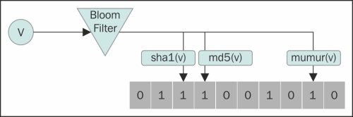
To add a key to a bloom filter (at the time of entering data in the associated collection), k hashes are calculated using k predefined hash functions. A modulus of each hash value is taken using array length l, and the value at this array position is set to 1.
The following pseudo code shows what happens:
//calculate hash, mod it to get location in bit array
arrayIndex1 = md5(v) % arrayLength
arrayIndex2 = sha1(v) % arrayLength
arrayindex3 = murmur(v) % arrayLength

//set all those indexes to 1
bitArray[arrayIndex1] = 1
bitArray[arrayIndex2] = 1
bitArray[arrayIndex3] = 1
To query the existence of a key in the bloom filter, the process is similar. Take the key and calculate the predefined hash values. Take modulus of the hash values with the length of the bit array. Look into those locations. If it turns out that at least one of those array locations have a zero value in them, it is certain that this value was never inserted in this bloom filter, and hence, does not exist in the associated collection. On the other hand, if all values are 1s, this means that the value may exist in the collection associated with this bloom filter. We cannot guarantee its presence in the collection because it is possible that there exist other k keys whose ith hash function filled the same spot in the array as the jth hash of the key that we are looking for.
Removal of a key from a bloom filter as in its original avatar is not possible. One may break multiple keys because multiple keys may have the same index bit set to 1 in the array for different hashes. Counting bloom filter solves these issues by changing the bit array into an integer array where each element works as a counter; insertion increments the counter and deletion decrements it.
Effectiveness of the bloom filter depends on the size of the collection it is applied to. The bigger the collection associated with the bloom filter, the higher the frequency of false positives will be (because the array will be more densely packed with 1s). Another thing that governs bloom filter is the quality of a good hash function. A good hash function will distribute hash values evenly in the array, and it will be fast. One does not look at the cryptic strength of the hash function here, so the Murmur3 hash will be preferred over the SHA1 hash.
From Cassandra 1.2 onwards, bloom filters are stored off heap memory. This is done to alleviate pressure on heap memory because Java garbage collectors start to underperform for heap size 8 GB or more, and that affects Cassandra's performance.
Index files are companion files of SSTables. Similar to the bloom filter, there exists one index file per SSTable. It contains all the row keys in the SSTable and its offset is at the point where the row starts in the data file.
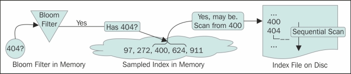
At startup, Cassandra reads every 128th key (configurable) into the memory (sampled index). When the index is looking for a row key (after the bloom filter hinted that the row key might be in this SSTable), Cassandra performs a binary search on the sampled index in memory. Followed by a positive result from the binary search, Cassandra will have to read a block in the index file from the disk starting from the nearest value lower than the value that we are looking for.
Let's take an example. See the figure in the Read repair and anti-entropy section, where Cassandra is looking for a row key 404. It is not in MemTable. On querying the bloom filter of a certain SSTable, Cassandra gets a positive nod that this SSTable may contain the row. The next step is to look into the SSTable. But before we start scanning the SSTable or the index file, we can get some help from the sampled index in memory. Looking through the sampled index, Cassandra finds out that there exists a row key 400 and another, 624. So, the row fragments may be in this SSTable. But more importantly, the sampled index tells the offset about the 400 entry in the index file. Cassandra now scans the SSTable from 400 and gets to the entry for 404. This tells Cassandra the offset of the entry for the 404 key in SSTable and it reads from there. The following figure shows the Cassandra SSTable index in action:
If you followed the example, you must have observed that the smaller the sampling size, the more the number of keys in the memory; the smaller the size of the block to read on the disk, the faster the results. This is a trade-off between memory usage and performance.
As we discussed earlier in the Read in action section, a read require may require Cassandra to read across multiple SSTables to get a result. This is wasteful, costs multiple (disk) seeks, may require a conflict resolution, and if there are too many SSTables, it may slow down the read. To handle this problem, Cassandra has a process in place, namely compaction. Compaction merges multiple SSTable files into one. Off the shelf, Cassandra offers two types of compaction mechanisms: size-tiered compaction strategy and level compaction strategy (refer to the Read performance section in Chapter 5, Performance Tuning). This section stays focused on a size-tiered compaction mechanism for better understanding.
The compaction process starts when the number of SSTables on disk reaches a certain threshold (configurable). Although the merge process is a little I/O intensive, it benefits in the long term with a lower number of disk seeks during reads. Apart from this, there are a few other benefits of compaction, as follows:
- Removal of expired tombstones (Cassandra v0.8+)
- Merging row fragments
- Rebuilds primary and secondary indexes
Merge is not as painful as it may seem because SSTables are already sorted. (Remember merge-sort?) Merge results into larger files, but old files are not deleted immediately. For example, let's say you have a compaction threshold set to four. Cassandra initially creates SSTables of the same size as MemTable. When the number of SSTables surpasses the threshold, the compaction thread triggers. This compacts the four equal-sized SSTables into one. Temporarily, you will have two times the total SSTable data on your disk. Another thing to note is that SSTables that get merged have the same size. So, when the four SSTables get merged to give a larger SSTable of size, say G, the buckets for the rest of the to-be-filled SSTables will be G each. So, the next compaction will take an even larger space while merging.
The SSTables, after merging, are marked as deletable. They get deleted at a garbage collection cycle of the JVM, or when Cassandra restarts.
The compaction process happens on each node and does not affect other nodes. This is called minor compaction. This is automatically triggered, system controlled, and regular. There is more than one type of compaction setting that exists in Cassandra. Another league of compaction is called, obviously, major compaction.
What's a major compaction? A major compaction takes all the SSTables, and merges them into one single SSTable. It is somewhat confusing when you see that a minor compaction merges SSTables and a major one does it too. There is a slight difference. For example, if we take the size-tiered compaction strategy, it merges the tables of the same size. So, if your threshold is four, Cassandra will start to merge when it finds four same sized SSTables. If your system starts with four SSTables of size X, after the compaction you will end up with one SSTable of size 4X. Next time when you have four X-sized SSTables, you will end up with two 4X tables, and so on. (These larger SSTables will get merged after 16 X-sized SSTables get merged into four 4X tables.) After a really long time, you will end up with a couple of really big SSTables, a handful of large SSTables, and many smaller SSTables. This is a result of continuous minor compaction. So, you may need to hop a couple of SSTables to get data for a query. Then, you run a major compaction and all the big and small SSTables get merged into one. This is the only benefit of major compaction.
Note
Major compaction may not be the best idea after Cassandra v0.8+. There are a couple of reasons for this. One reason is that automated minor compaction no longer runs after a major compaction is executed. So, this adds up manual intervention or doing extra work (such as setting a cron job) to perform regular major compaction. The performance gain after major compaction may deteriorate with time. Probably because of the larger the SSTable, which is what we get after major compaction, it is more likely to get more bloom filter false positive. And then, it will take longer to perform binary search on the index, which is very big.
Cassandra is a complex system with its data distributed among commit logs, MemTables, and SSTables on a node. The same data is then replicated over replica nodes. So, like everything else in Cassandra, deletion is going to be eventful. Deletion, to an extent, follows an update pattern, except Cassandra tags the deleted data with a special value, and marks it as a tombstone. This marker helps future queries, compaction, and conflict resolution. Let's step further down and see what happens when a column from a column family is deleted.
A client connected to a node (a coordinator node may not be the one holding the data that we are going to mutate), issues a delete command for a column C, in a column family CF. If the consistency level is satisfied, the delete command gets processed. When a node, containing the row key receives a delete request, it updates or inserts the column in MemTable with a special value, namely tombstone. The tombstone basically has the same column name as the previous one; the value is set to the Unix epoch. The timestamp is set to what the client has passed. When a MemTable is flushed to SSTable, all tombstones go into it as any regular column will.
On the read side, when the data is read locally on the node and it happens to have multiple versions of it in different SSTables, they are compared and the latest value is taken as the result of reconciliation. If a tombstone turns out to be a result of reconciliation, it is made a part of the result that this node returns. So, at this level, if a query has a deleted column, this exists in the result. But the tombstones will eventually be filtered out of the result before returning it back to the client. So, a client can never see a value that is a tombstone.
For consistency levels more than one, the query is executed on as many replicas as the consistency level. The same as a regular read process, data from the closest node and a digest from the remaining nodes is obtained (to satisfy the consistency level). If there is a mismatch, such as the tombstone not yet being propagated to all the replicas, a partial read repair is triggered, where the final view of the data is sent to all the nodes that were involved in this read, to satisfy the consistency level.
One thing where delete differs from update is a compaction. A compaction removes a tombstone only if its (the tombstone's) garbage collection's grace seconds (t) are over. This t is called gc_grace_seconds (configurable). So, do not expect that a major deletion will free up a lot of space immediately.
What happens to a node that was holding data that was deleted (in other live replicas) when this node was down? If a tombstone still exists in any of the replica nodes, the delete information will eventually be available to the previously dead node. But a compaction occurs at gc_grace_seconds, after the deletion will kick the old tombstones out. This is a problem, because no information about the deleted column is left. Now, if a node that was dead all the time during gc_grace_seconds wakes up and sees that it has some data that no other node has, it will treat this data as fresh data, and assuming a write failure, it will replicate the data over all the other replica nodes. The old data will resurrect and replicate, and may reappear in client results.
gc_grace_seconds is 10 days by default, before which any sane system admin will bring the node back in, or discard the node completely. But it is something to watch out for and repair nodes occasionally.
When we last talked about durability, we observed that Cassandra provides a commit log to provide write durability. This is good. But what if the node, where the writes are going to be, is itself dead? No communication will keep anything new to be written to the node. Cassandra, inspired by Dynamo, has a feature called "hinted handoff". In short, it's the same as taking a quick note locally that X cannot be contacted; here is the mutation, M, that will be required to be replayed when it comes back.
The coordinator node (the node which the client is connected to) on receipt of a mutation/write request forwards it to appropriate replicas that are alive. If this fulfills the expected consistency level, the write is assumed successful. The write requests a node that does not respond to a write request or is known to be dead (via gossip) and is stored locally in the system.hints table. This hint contains the mutation. When a node comes to know, via gossip, that a node is recovered, it replays all the hints it has in store for that node. Also, every 10 minutes, it keeps checking any pending hinted handoffs to be written.
Why worry about hinted hand off when you have written to satisfy the consistency level? Wouldn't it eventually get repaired? Yes, that's right. Also, hinted handoff may not be the most reliable way to repair a missed write. What if the node that has hinted handoff dies? This is a reason we do not count on hinted handoff as a mechanism to provide consistency (except for the case of the consistency level, ANY) guarantee; it's a single point of failure. The purposes of hinted handoff are one- to make restored nodes quickly consistent with the other live ones; and two to provide extreme write availability when consistency is not required.
The way extreme write availability is obtained is at the cost of consistency. One can set consistency level for writes to ANY. What happens next is that if all the replicas that are meant to hold this value are down, Cassandra will just write a local hinted handoff and return write success to the client. There is one caveat; the handoff can be on any node. So, a read for the data that we have written as a hint will not be available as long as the replicas are dead plus until the hinted handoff is replayed. But it is a nice feature.
Note
There is a slight difference where hinted handoff is stored in Cassandra's different versions. Prior to Cassandra 1.0, hinted handoff is stored on one of the replica nodes that can be communicated with. From Version 1.0+ (including 1.0), handoff can be written on the coordinator node (the node that the client is connected to).
Removing a node from a cluster causes deletion of hinted handoff stored for that node. All hints for deleted records are dropped.
Cassandra promises eventual consistency and read repair is the process that does this part. Read repair, as the name suggests, is the process of fixing inconsistencies among the replicas at the time of read. What does that mean? Let's say we have three replica nodes, A, B, and C, that contain a data X. During an update, X is updated to X1 in replicas A and B, but it fails in replica C for some reason. On a read request for data X, the coordinator node asks for a full read from the nearest node (based on the configured snitch) and digest of data X from other nodes to satisfy consistency level. The coordinator node compares these values (something like digest(full_X) == digest_from_node_C). If it turns out that the digests are the same as the digests of the full read, the system is consistent and the value is returned to the client. On the other hand, if there is a mismatch, full data is retrieved and reconciliation is done and the client is sent the reconciled value. After this, in the background, all the replicas are updated with the reconciled value to have a consistent view of data on each node. The following figure shows this process:
- Client queries for data X, from a node C (coordinator)
- C gets data from replicas R1, R2, and R3 reconciles
- Sends reconciled data to client
- If there is a mismatch across replicas, a repair is invoked
The following figure shows the read repair dynamics:
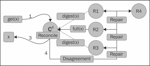
So, we have got a consistent view on read. What about the data that is inserted, but never read? Hinted handoff is there, but we do not rely on hinted handoff for consistency. What if the node containing hinted handoff data dies, and the data that contains the hint is never read? Is there a way to fix them without read? This brings us to the anti-entropy architecture of Cassandra (borrowed from Dynamo).
Anti-entropy compares all the replicas of a column family and updates the replicas to the latest version. This happens during major compaction. It uses Merkle trees to determine discrepancies among the replicas and fixes them.
Merkle tree is a hash tree where leaves of the tree hashes hold actual data in column family and non-leaf nodes hold hashes of their children. For more information, refer to A digital signature Based On A Conventional Encryption Function by Merkle, R. (1988), available at http://link.springer.com/chapter/10.1007%2F3-540-48184-2_32. The unique advantage of a Merkle tree is that a whole subtree can be validated just by looking at the value of the parent node. So, if nodes on two replica servers have the same hash values, then the underlying data is consistent and there is no need to synchronize. If one node passes the whole Merkle tree of a column family to another node, it can determine all the inconsistencies.
The following figure shows the Merkle tree to determine a mismatch in hash values at the parent nodes due to the difference in the underlying data:
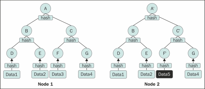
To exemplify this, the preceding figure shows the Merkle tree from two nodes with inconsistent data. A process comparing these two trees would know that there is something inconsistent, because the hash values stored in the top nodes do not match. It can descend down and knows that the right subtree is likely to have an inconsistency. And then, the same process is repeated until it finds out that all the data is mismatched.