
Cassandra is all about speed—quick installation, fast reads, and fast writes. You got your application optimized, minimized the network trips by batching, and denormalized the data to get maximum information in one request. However, the performance is not what you read over the Web and in various blogs. You start to doubt whether the claims actually measure. Hold on! You may need to tune things up.
This chapter will discuss how to get a sense of a Cassandra cluster's capacity and have a performance number handy to back up our claims. It then dives into the various settings that affect read and write throughput, a couple of JVM tuning parameters, and finally, a short discussion on how scaling systems horizontally and vertically can improve the performance.
Before you start to claim the performance numbers of your Cassandra backend, based on numbers that you have read elsewhere, it is important to perform your own stress testing. It is very easy to do that in Cassandra, as it provides special tools for stress testing. It is a good idea to customize the parameters of the stress test, which represents a use case that is closer to what your application is going to do. This will save a lot of heated discussion later, due to discrepancies in the load testing and the actual throughput that the software is able to pull out of the setting.
Cassandra 2.1 ships with very sophisticated stress test tools that can be fine-tuned to simulate the expected load on the system and can help to measure Cassandra's performance under stress conditions. To create a load scenario, you need to set up a YAML file that specifies the four things: database schema, data distribution, write pattern, and read queries.
You need to provide the keyspace name, the keyspace creation query, the table name that is to be stressed, and the table creation query.
You can provide the pattern of the data you are expecting in your application, and their spread across a partition key. So, basically, you choose the following:
- Size: This shows the statistical distribution of the size of data in a column. For example, for the e-mail address, I would like a 3 to 15 character column with normal distribution. So, the mean e-mail address length would be 9–10 characters, which seems reasonable. The default value is
UNIFORM(4..8). - Population: This shows the unique column values, and how they are distributed. For example, for a
citycolumn, I would opt for 20,000 unique values. Also assuming that most of the records belong to just a few cities, for example 20 percent of cities account for 80 percent of records, we want some sort of diminishing distribution. Therefore, we would like to choose exponential distribution across rows for the city column. The default value isUNIFORM(1..100B). - Cluster: If you are using a composite key, there are probable chances that you have more than one record for a given row-key partition key. The
clusteringattribute defines how the cluster size varies. For example, whether you wanted to fix the number of rows for a given partition key or you wanted to have some kind of variation. The default value isFIXED(1).
The stress tool provides six types of statistical distributions. They are as follows:
FIXED(value): This distribution always returns the same value as specified by the argumentGAUSSIAN(min..max, mean, standard_deviation): Normal distribution over[min, max]with mean asmeanandstandard_deviationGAUSSIAN(min..max, standard_deviation_range): Gaussian distribution over[min, max]with mean at(min+max)/2andstandard_deviationas(mean-min)/standard_deviation_rangeUNIFORM(min..max): Uniform distribution over[min, max]EXP(min..max): Exponential distribution over the range[min, max]EXTREME(min..max, shape): Weibull distribution over the range[min, max]
When writing data, you can specify how it should be distributed across the rows and clusters. There are four things that may be specified as follows:
- Partitions: This attribute specifies the distribution of the
INSERTqueries in each batch across all partitions (clusters). The default isFIXED(1), which means one value per partition per batch. - Pervisit: This shows the ratio of rows that goes into a partition; this ratio is proportional to the total number of rows for the partition. If you have a secondary key column distribution as
FIXED(20000), thenFIXED(1)/2000will denote that each batch will insert 10 rows. If not specified, it defaults toFIXED(1)/1. - Perbatch: This shows the ratio of rows each partition should update in a single batch, as a proportion of the number of rows picked by the pervisit ratio and partition count. The default is
FIXED(1). - Batchtype: By default, the stress test uses the
LOGGEDbatches. One may set it asUNLOGGEDfor better performance.
A map (JSON) of queries with the key being its name, and the value is the query itself. The query may have parameters to be filled later by the stress tool.
An example YAML looks like the following (taken from https://gist.github.com/tjake/fb166a659e8fe4c8d4a3; you can find the gist on my GitHub account https://gist.github.com/naishe/f7c7090173f4ea6afc28):
#1: Database Schema
# Keyspace Name
keyspace: stresscql

keyspace_definition: |
  CREATE KEYSPACE stresscql WITH replication = {'class': 'SimpleStrategy', 'replication_factor': 1};

# Table name
table: blogposts

# The CQL for creating a table you wish to stress (optional if it already exists)
table_definition: |
  CREATE TABLE blogposts (
        domain text,
        published_date timeuuid,
        url text,
        author text,
        title text,
        body text,
        PRIMARY KEY(domain, published_date)
  ) WITH CLUSTERING ORDER BY (published_date DESC)
    AND compaction = { 'class':'LeveledCompactionStrategy' }
    AND comment='A table to hold blog posts';

#2: Data Distribution
columnspec:
  - name: domain size: gaussian(5..100) population: uniform(1..10M)

  - name: published_date cluster: fixed(1000)

  - name: url size: uniform(30..300)

  - name: title size: gaussian(10..200)

  - name: author size: uniform(5..20)

  - name: body size: gaussian(100..5000)

#3: Write pattern

insert:
  partitions: fixed(1)
  pervisit:  fixed(1)/1000
  perbatch:  fixed(1)/1
  batchtype: UNLOGGED

#4: Read pattern
queries:
   singlepost:  select * from blogposts where domain = ? LIMIT 1
   timeline: select url, title, published_date from blogposts where domain = ? LIMIT 10
This stress test was executed on an all default Cassandra 2.1.0 clusters, with the following specifications (AWS i2.xlarge instances):
Number of machines: 3 (3*256 Virtual nodes)
RAM: 30GB
Storage: 800GB SSD
CPU cores: 4 (virtualized)
To find the test result, run the following command:
$ CASSANDRA_HOME/tools/bin/cassandra-stress user profile=blogpost.yaml ops(insert=1)
[ -- snip -- ]
Results:
op rate                   : 9397
partition rate            : 9397
row rate                  : 9393
latency mean              : 28.7
latency median            : 17.2
latency 95th percentile   : 94.8
latency 99th percentile   : 173.9
latency 99.9th percentile : 572.1
latency max               : 791.6
Total operation time      : 00:00:37
The following screenshot shows the test results:
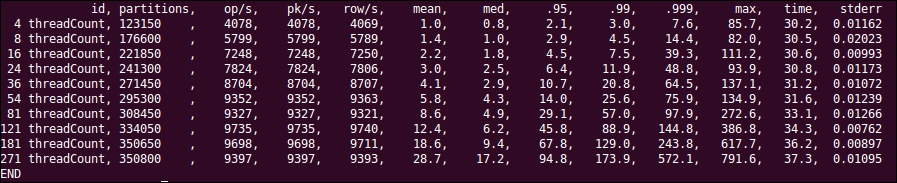
Although 9,000 writes per second is not the most terrible thing from three expensive machines, it may need a bit tweaking to try to perform better. The rest of this chapter will talk about various settings within Cassandra and JVM to boost the performance for the given use case.