
H2O Flow is a web-based open source user interface for H2O and, given that it is being used with Spark, Sparkling Water. It is a fully functional H2O web interface for monitoring the H2O Sparkling Water cluster jobs, and also for manipulating data and training models.
We have created some simple example code to start the H2O interface. As in the previous Scala-based code samples, all we need to do is create a Spark, an H2O context, and then call the openFlow command, which will start the Flow interface.
The following Scala code example just imports classes for Spark context, configuration, and H2O. It then defines the configuration in terms of the application name and the Spark cluster URL.
A Spark context is then created using the configuration object:
import org.apache.spark.SparkContext
import org.apache.spark.SparkContext._
import org.apache.spark.SparkConf
import org.apache.spark.h2o._

object h2o_spark_ex2  extends App {
   val sparkMaster = "spark://localhost:7077"
   val appName = "Spark h2o ex2"
   val conf = new SparkConf()

   conf.setMaster(sparkMaster)
   conf.setAppName(appName)

   val sparkCxt = new SparkContext(conf)
An H2O context is then created and started using the Spark context. The H2O context classes are imported, and the Flow user interface is started with the openFlow command:
  implicit val h2oContext = new org.apache.spark.h2o.H2OContext(sparkCxt).start()

   import h2oContext._

   // Open H2O UI

   openFlow
Note that, for the purposes of this example and to enable us to use the Flow application, we have commented out the H2O shutdown and the Spark context stop options. We would not normally do this, but we wanted to make this application long-running so that it gives us plenty of time to use the interface:
  // shutdown h20

 //  water.H2O.shutdown()
 //  sparkCxt.stop()

   println( " >>>>> Script Finished <<<<< " )

 } // end application
We use our Bash script run_h2o.bash with the application class name called h2o_spark_ex2 as a parameter. This script contains a call to the spark-submit command, which will execute the compiled application:
[hadoop@hc2r1m2 h2o_spark_1_2]$ ./run_h2o.bash h2o_spark_ex2
When the application runs, it lists the state of the H2O cluster and provides a URL by which the H2O Flow browser can be accessed:
15/05/20 13:00:21 INFO H2OContext: Sparkling Water started, status of context:
 Sparkling Water Context:
  * number of executors: 4
  * list of used executors:
   (executorId, host, port)
   ------------------------
   (1,hc2r1m4,54321)
   (3,hc2r1m2,54321)
   (0,hc2r1m3,54321)
   (2,hc2r1m1,54321)
   ------------------------
Open H2O Flow in browser: http://192.168.1.108:54323 (CMD + click in macOS).
The previous example shows that we can access the H2O interface using the port number 54323 on the host IP address 192.168.1.108.
So, we can access the interface using the hc2r1m2:54323 URL. The following screenshot shows the Flow interface with no data loaded.
There are data processing and administration menu options, and buttons at the top of the page. To the right, there are help options to enable you to learn more about H2O:

The following screenshot shows the menu options and buttons in greater detail. In the following sections, we will use a practical example to explain some of these options, but there will not be enough space in this chapter to cover all the functionality. Check the http://h2o.ai/ website to learn about the Flow application in detail, available at http://h2o.ai/product/flow/:

In greater definition, you can see that the previous menu options and buttons allow you to both administer your H2O Spark cluster and also manipulate the data that you wish to process.
The following screenshot shows a reformatted list of the help options available, so that if you get stuck, you can investigate solving your problem from the same interface:

If we go to Menu | Admin | Cluster Status, we will obtain the following screenshot, which shows us the status of each cluster server in terms of memory, disk, load, and cores.
It's a useful snapshot that provides us with a color-coded indication of the status:

The menu option, Admin | Jobs, provides details of the current cluster jobs in terms of the start, end, runtimes, and status. Clicking on the job name provides further details, as shown next, including data processing details and an estimated runtime, which is useful. Also, if you select the Refresh button, the display will continuously refresh until it is deselected:

The Admin | Water Meter option provides a visual display of the CPU usage on each node in the cluster.
As you can see in the following screenshot, our meter shows that my cluster was idle:

Using the menu option, Flow | Upload File, we have uploaded some of the training data used in the previous Deep Learning Scala-based example.
The data has been loaded into a data preview pane; we can see a sample of the data that has been organized into cells. Also, an accurate guess has been made of the data types so that we can see which columns can be enumerated. This is useful if we want to consider classification:

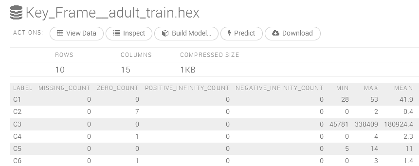
Having loaded the data, we are now presented with a Frame display, which offers us the ability to view, inspect, build a model, create a prediction, or download the data. The data display shows information such as min, max, and mean.
It shows data types, labels, and a zero data count, as shown in the following screenshot:
We thought that it would be useful to create a Deep Learning classification model based on this data to compare the Scala-based approach to this H2O user interface. Using the view and inspect options, it is possible to visually and interactively check the data, as well as create plots relating to the data. For instance, using the previous inspect option followed by the plot columns option, we were able to create a plot of data labels versus zero counts in the column data. The following screenshot shows the result:

By selecting the Build Model option, a menu option is offered that lets us choose a model type. We will select deeplearning, as we already know that this data is suited to this classification approach.
The previous Scala-based model resulted in an accuracy level of 83 percent:

We have selected the deeplearning option. Having chosen this option, we are able to set model parameters such as training and validation Datasets, as well as choose the data columns that our model should use (obviously, the two Datasets should contain the same columns).
The following screenshot displays the Datasets and the model columns being selected:

There is a large range of basic and advanced model options available. A selection of them is shown in the following screenshot.
We have set the response column to 15 as the income column. We have also set the VARIABLE_IMPORTANCES option. Note that we don't need to enumerate the response column, as it has been done automatically:

Note also that the epochs or iterations option is set to 100, as before. Also, the figure 200, 200 for the hidden layers indicates that the network has two hidden layers, each with 200 neurons. Selecting the Build Model option causes the model to be created with these parameters.
The following screenshot shows the model being trained, including an estimation of training time and an indication of the data processed so far:

Viewing the model, once trained, shows training and validation metrics, as well as a list of the important training parameters:

Selecting the Predict option allows an alternative validation Dataset to be specified. Choosing the Predict option using the new Dataset causes the already trained model to be validated against a new test Dataset:

Selecting the Predict option causes the prediction details for the DeepLearning model and the Dataset to be displayed, as shown in the following screenshot:

The preceding screenshot shows the test data frame and the model category, as well as the validation statistics in terms of AUC, GINI, and MSE.
The AUC value, or area under the curve, relates to the ROC, or the receiver operator characteristics curve, which is also shown in the following screenshot.
TPR means True Positive Rate, and FPR means False Positive Rate.
AUC is a measure of accuracy, with a value of one being perfect. So, the blue line shows greater accuracy than that of the red line, which is basically random guessing:

There is a great deal of functionality available within this interface that we have not explained, but we hope that we have given you a feel for its power and potential. You can use this interface to inspect your data and create reports before attempting to develop code, or as an application in its own right to delve into your data.