
Part 4
3D Modeling and Imaging
- Chapter 21: Creating 3D Drawings
- Chapter 22: Using Advanced 3D Features
- Chapter 23: Rendering 3D Drawings
- Chapter 24: Editing and Visualizing 3D Solids
- Chapter 25: Exploring 3D Mesh and Surface Modeling
Chapter 21
Creating 3D Drawings
Viewing an object in three dimensions gives you a sense of its true shape and form. It also helps you conceptualize your design, which results in better design decisions. In addition, using three-dimensional objects helps you communicate your ideas to those who may not be familiar with the plans, sections, and side views of your design.
A further advantage to drawing in three dimensions is that you can derive 2D drawings from your 3D models, which may take considerably less time than creating them with standard 2D drawing methods. For example, you can model a mechanical part in 3D and then quickly derive its 2D top, front, and right-side views by using the techniques discussed in this chapter.

The AutoCAD LT® software does not support any of the 3D-related features described in this chapter.
In this chapter, you will learn to:
- Know the 3D Modeling workspace
- Draw in 3D using solids
- Create 3D forms from 2D shapes
- Isolate coordinates with point filters
- Move around your model
- Get a visual effect
- Turn a 3D view into a 2D AutoCAD drawing
Getting to Know the 3D Modeling Workspace
Most of this book is devoted to showing you how to work in the Drafting & Annotation workspace. This workspace is basically a 2D drawing environment, although you can certainly work in 3D as well.
The AutoCAD® 2014 program offers the 3D Modeling and 3D Basics workspaces, which give you a set of tools to help ease your way into 3D modeling. The 3D Modeling workspace gives AutoCAD a different set of Ribbon panels, but don’t worry. AutoCAD behaves in the same basic way, and the AutoCAD files produced are the same regardless of whether they’re 2D or 3D drawings.
The 3D Basics workspace contains the minimum 3D tools needed to perform 3D functions.
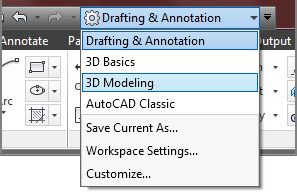
To get to the 3D Modeling workspace, you need to click the Workspace tool in the Quick Access toolbar and then select 3D Modeling (see Figure 21-1).
Figure 21-1 The Workspace tool
If you’re starting a new 3D model, you’ll also want to create a new file using a 3D template. Try the following to get started with 3D modeling:
Figure 21-2 The AutoCAD 3D Modeling workspace
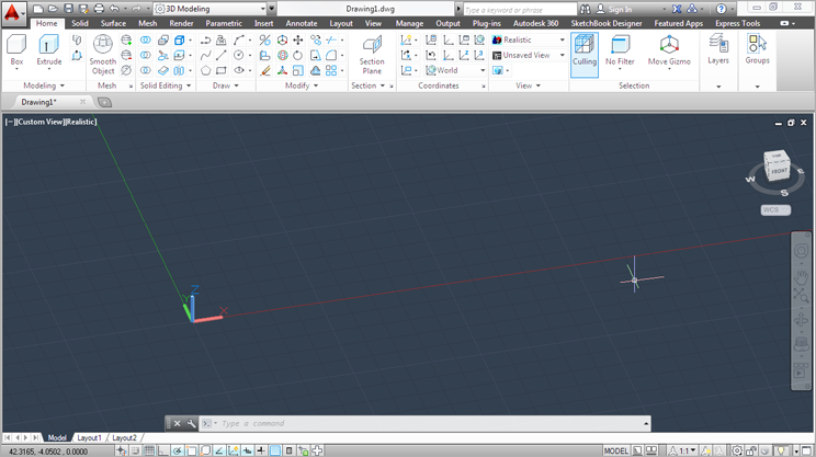
The drawing area displays the workspace as a perspective view with a dark gray background and a grid. This is just a typical AutoCAD drawing file with a couple of setting changes. The view has been set up to be a perspective view by default, and a feature called Visual Styles has been set to Realistic, which will show 3D objects as solid objects. You’ll learn more about the tools you can use to adjust the appearance of your workspace later in this chapter. For now, let’s look at the tool palette and Ribbon that appear in the AutoCAD window.
To the far right is the AutoCAD Materials Browser palette. It shows a graphical list of surface materials that you can easily assign to 3D objects in your model. If the Materials Browser does not open by default, you’ll see how to open it and learn more about materials in Chapter 23, “Rendering 3D Drawings.”
The Ribbon along the top of the AutoCAD window offers all the tools you’ll need to create 3D models. The 3D Modeling workspace Ribbon offers a few of the tabs and panels with which you’re already familiar, but many of the tabs will be new to you (see Figure 21-3). You see the familiar Draw and Modify panels in the Home tab, but there are several other panels devoted to 3D modeling: Modeling, Mesh, Solid Editing, Section, Coordinates, View, and Selection.
Figure 21-3 Some of the Ribbon tabs and panels of the 3D Modeling workspace
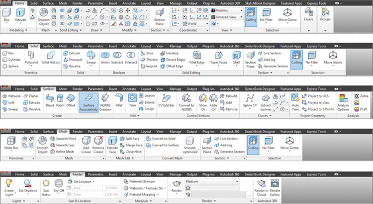
In addition, other Ribbon tabs offer more sets of tools designed for 3D modeling. For example, the Render tab contains tools that control the way the model looks. You can set up lighting and shadows and apply materials to objects such as brick or glass. You can also control the way AutoCAD illuminates the model through the Lights, Sun & Location, and Materials panels. In the next section, you’ll gain firsthand experience creating and editing some 3D shapes using the Home tab’s Modeling and View panels and the View tab’s Visual Styles panel. This way, you’ll get a feel for how things work in the 3D Modeling workspace.
Drawing in 3D Using Solids
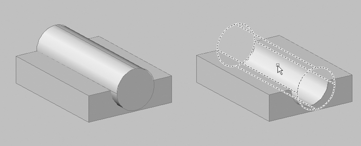
You can work with three types of 3D objects in AutoCAD: solids, surfaces, and mesh objects. You can treat solid objects as if they’re solid material. For example, you can create a box and then remove shapes from the box as if you’re carving it, as shown in Figure 21-4.
Figure 21-4 Solid modeling lets you remove or add shapes.
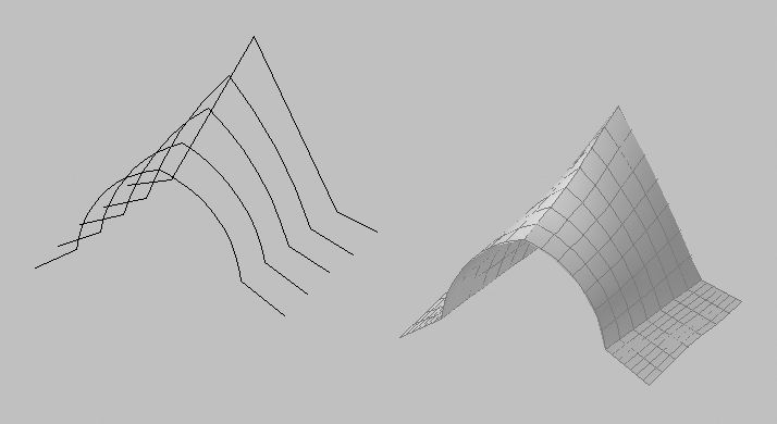
With surfaces, you create complex surface shapes by building on lines, arcs, or polylines. For example, you can quickly turn a series of curved polylines, arcs, or lines into a warped surface, as shown in Figure 21-5.
A mesh object is made up of edges, faces, and vertices. These basic parts create a series of square or triangular areas to define a three-dimensional form. Mesh objects can be created with primitives in the same way solid primitives can. Their behavior is different, though. Mesh objects do not have mass properties like solids, but they can be altered through free-form modeling techniques. Creases as well as splits can be added to the forms. The level of smoothness can be altered, which means you can add more edges, faces, and vertices to create a more rounded and organic-looking object.
Figure 21-5 Using the Loft tool, you can use a set of 2D objects (left) to define a complex surface (right).
Next, you’ll learn how to create a solid box and then make simple changes to it as an introduction to 3D modeling.
Adjusting Appearances
Before you start to work on the exercises, you’ll want to change the visual style to one that will make your work a little easier to visualize in the creation phase. Visual Styles offers a way to let you see your model in different styles, from sketch-like to realistic. You’ll learn more about Visual Styles in the section “Getting a Visual Effect” later in this chapter. For now, you’ll get a brief introduction by changing the style for the exercises that follow:
Creating a 3D Box
Start by creating a box using the Box tool in the Home tab’s Modeling panel:
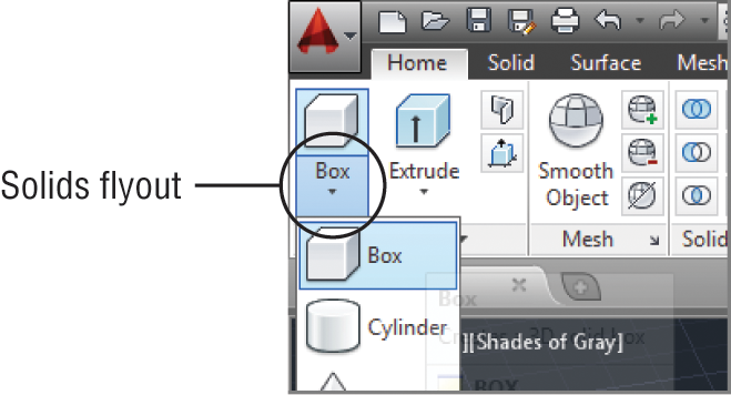
Figure 21-6 Drawing a 3D solid box
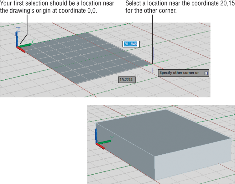
You used three basic steps in creating the box. First, you clicked one corner to establish a location for the box. Then, you clicked another corner to establish the base size. Finally, you selected a height. You use a similar set of steps to create any of the other 3D solid primitives found in the Solids flyout of the Home tab’s Modeling panel. For example, for a cylinder, you select the center, then the radius, and finally the height. For a wedge, you select two corners as you did with the box, and then you select the height. You’ll learn more about these 3D solid primitives in Chapter 24, “Editing and Visualizing 3D Solids.”
Editing 3D Solids with Grips
Once you’ve created a solid, you can fine-tune its shape by using grips:
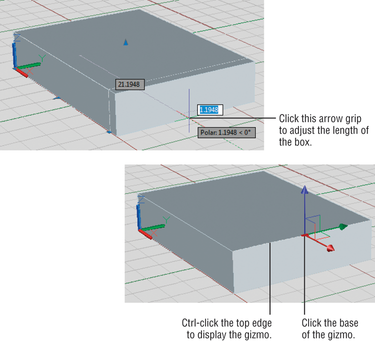
Figure 21-7 Grips appear on the 3D solid.
Constraining Motion with the Gizmo
You can move individual edges by using a Ctrl+click. This will activate the gizmo. The gizmo is an icon that looks like the UCS icon and appears whenever you select a 3D solid or any part of a 3D solid. Try the next exercise to see how it works:
Figure 21-8 Using the gizmo to constrain motion
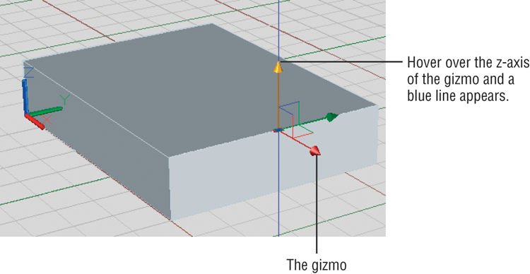
Here you used the gizmo to change the Z location of a grip easily. You can use the gizmo to modify the location of a single grip or the entire object.
Rotating Objects in 3D Using Dynamic UCS
Typically, you work in what is known as the World Coordinate System (WCS). This is the default coordinate system that AutoCAD uses in new drawings, but you can also create your own coordinate systems that are subsets of the WCS. A coordinate system that you create is known as a User Coordinate System (UCS).
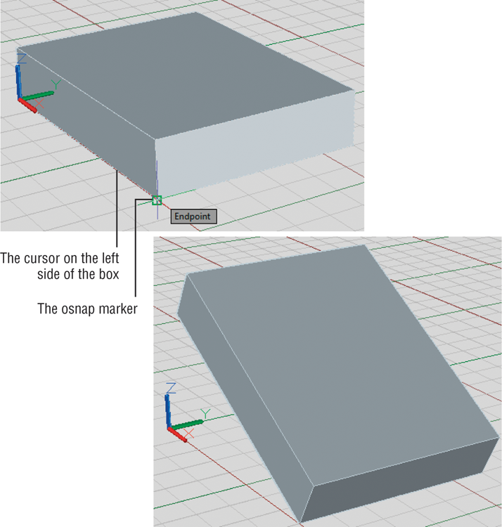
UCSs are significant in 3D modeling because they can help you orient your work in 3D space. For example, you could set up a UCS on a vertical face of the 3D box you created earlier. You could then draw on that vertical face just as you would on the drawing’s WCS. Figure 21-9 shows a cylinder drawn on the side of a box. If you click the Cylinder tool, for example, and place the cursor on the side of the box, the side will be highlighted to indicate the surface to which the cylinder will be applied. In addition, if you could see the cursor in color, you would see that the blue z-axis is pointing sideways to the left and is perpendicular to the side of the box.
The UCS has always been an important tool for 3D modeling in AutoCAD. The example just described demonstrates the Dynamic UCS, which automatically changes the orientation of the x-, y-, and z-axes to conform to the flat surface of a 3D object.
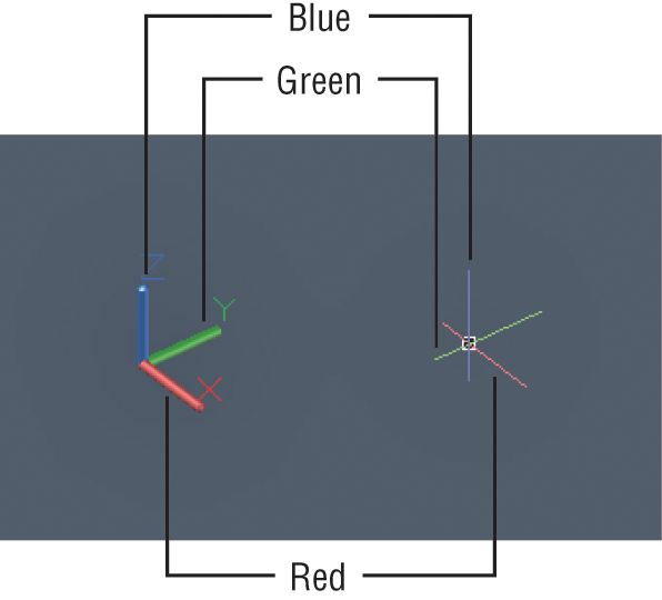
You may have noticed that when you created the new 3D file using the acad3D.dwt template, the cursor looked different. Instead of the usual cross, you saw three intersecting lines. If you look carefully, you’ll see that each line of the cursor is a different color. In its default configuration, AutoCAD shows a red line for the x-axis, a green line for the y-axis, and a blue line for the z-axis. This mimics the color scheme of the UCS icon, as shown in Figure 21-10.
Figure 21-9 Drawing on the side of a box
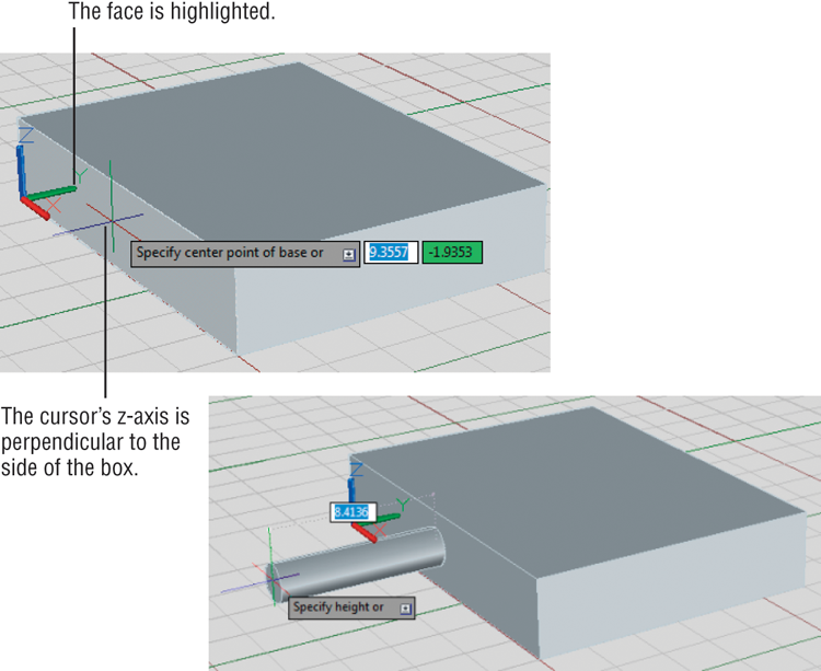
Figure 21-10 The UCS icon at the left and the cursor in 3D to the right are color matched.
As you work with the Dynamic UCS, you’ll see that the orientation of these lines changes when you point at a surface on a 3D object. The following exercise shows you how to use the Dynamic UCS to help you rotate the box about the x-axis:
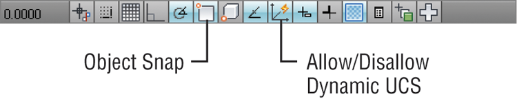
Figure 21-11 Selecting a base point, and the resulting box orientation
Here you saw that you could hover over a surface to indicate the plane about which the rotation is to occur. Now, suppose you want to add an object to one of the sides of the rotated box. The next section will show you another essential tool—one you can use to do just that.
Drawing on a 3D Object’s Surface
In the rotation exercise, you saw that you could hover over a surface to indicate the plane of rotation. You can use the same method to indicate the plane on which you want to place an object. Try the following exercise to see how it’s done:
Figure 21-12 Drawing circles on the surface of a 3D solid
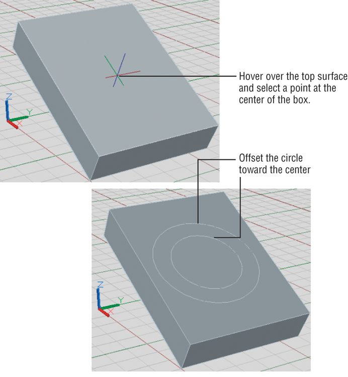
This demonstrates that you can use Dynamic UCS to align objects with the surface of an object. Note that Dynamic UCS works only on flat surfaces. For example, you can’t use it to place an object on the curved side of a cylinder.
Pushing and Pulling Shapes from a Solid
You’ve just added two 2D circles to the top surface of the 3D box. AutoCAD offers a tool that lets you use those 2D circles or any closed 2D shapes to modify the shape of your 3D object. The Presspull tool in the Home tab’s Modeling panel lets you “press” or “pull” a 3D shape to or from the surface of a 3D object. The following exercise shows how this works:
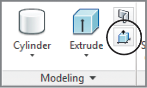
Figure 21-13 Move the cursor over different areas of the box and notice how the areas are highlighted.
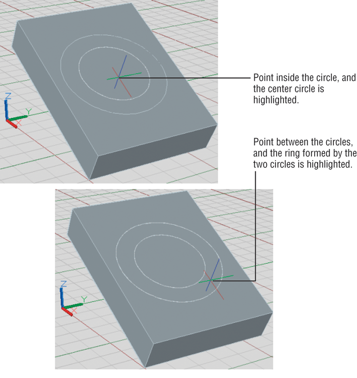
Figure 21-14 Creating an indentation in the box using Presspull

You’ve created a circular indentation in the box by pressing the circular area defined by the two circles. You could have pulled the area upward to form a circular ridge on the box. Pressing the circle into the solid is essentially the same as subtracting one solid from another. When you press the shape into the solid, AutoCAD assumes you want to subtract the shape.
Presspull works with any closed 2D shape, such as a circle, closed polyline, or other completely enclosed area. An existing 3D solid isn’t needed. For example, you can draw two concentric circles without the 3D box and then use Presspull to convert the circles into a 3D solid ring. In the previous exercise, the solid box showed that you can use Presspull to subtract a shape from an existing solid.
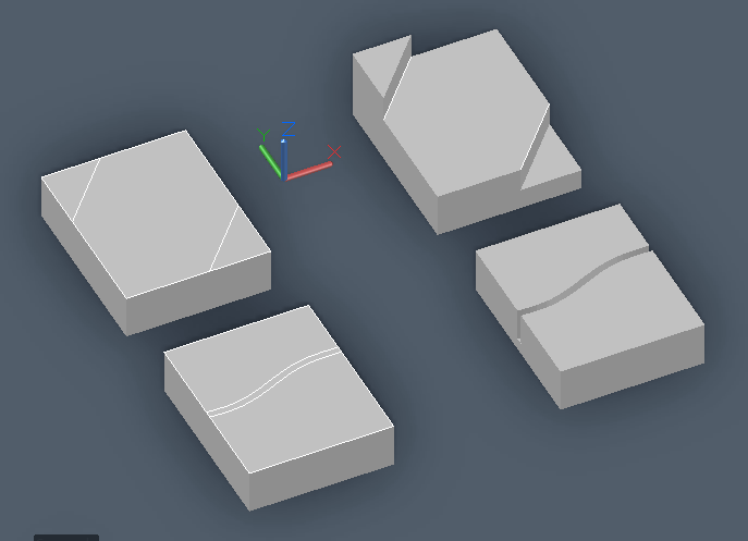
As you saw in this exercise, the Presspull tool can help you quickly subtract a shape from an existing 3D solid. Figure 21-15 shows some other examples of how you can use Presspull. For example, you can draw a line from one edge to another and then use Presspull to extrude the resulting triangular shape. You can also draw concentric shapes and extrude them; you can even use offset spline curves to add a trough to a solid.
Figure 21-15 Creating complex shapes using the Presspull tool
Making Changes to Your Solid
When you’re creating a 3D model, you’ll hardly ever get the shape right the first time. Suppose you decide that you need to modify the shape you’ve created so far by moving the hole from the center of the box to a corner. The next exercise will show you how you can gain access to the individual components of a 3D solid to make changes.
The model with which you’ve been working is composed of two objects: a box and a cylinder formed from two circles. These two components of the solid are referred to as subobjects of the main solid object. Faces and edges of 3D solids are also considered subobjects. When you use the Union, Subtract, and Intersect tools later in this book, you’ll see that objects merge into a single solid—or at least that is how it seems at first. You can gain access to and modify the shape of the subobjects from which the shape is constructed by using the Ctrl key while clicking the solid. Try the following:
Figure 21-16 You can select subobjects of a 3D solid when you hold down the Ctrl key.
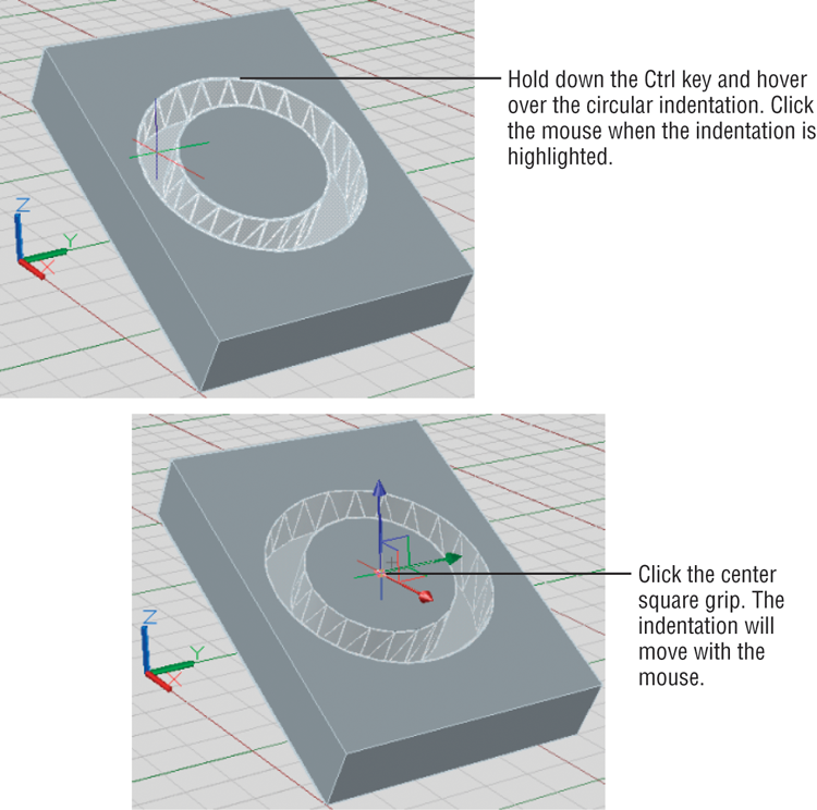
Figure 21-17 You can move the indentation to a new location using its grip.
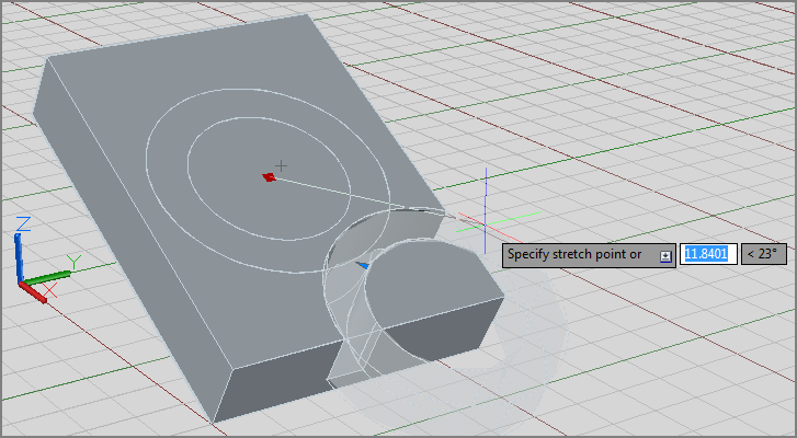
This example showed that the Ctrl key can be an extremely useful tool when you have to edit a solid; it allows you to select the subobjects that form your model. Once the subobjects are selected, you can move them, or you can use the arrow grips to change their size.
Creating 3D Forms from 2D Shapes
You’ve seen that 3D solid primitives are great for creating basic shapes, but in many situations you’ll want to create a 3D form from a more complex shape. Fortunately, you can extrude 2D objects into a variety of shapes using additional tools found in the Home tab’s Modeling panel. For example, you can draw a shape like a star and then extrude it along the z-axis, as shown in Figure 21-18. Alternatively, you can use several strategically placed 2D objects to form a flowing surface like the wing of an airplane.
Figure 21-18 The closed polyline on the left can be used to construct the 3D shape on the right.
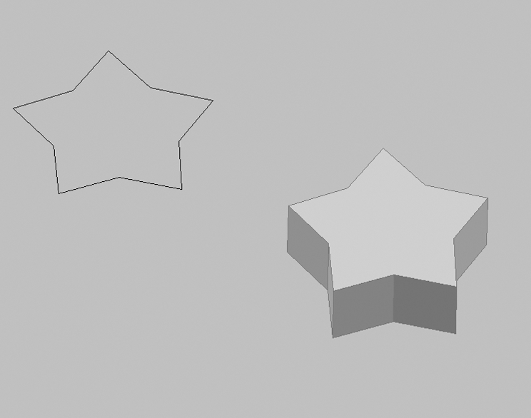
You can create a 3D solid by extruding a 2D closed polyline. This is a more flexible way to create shapes because you can create a polyline of any shape and extrude it to a fairly complex form.
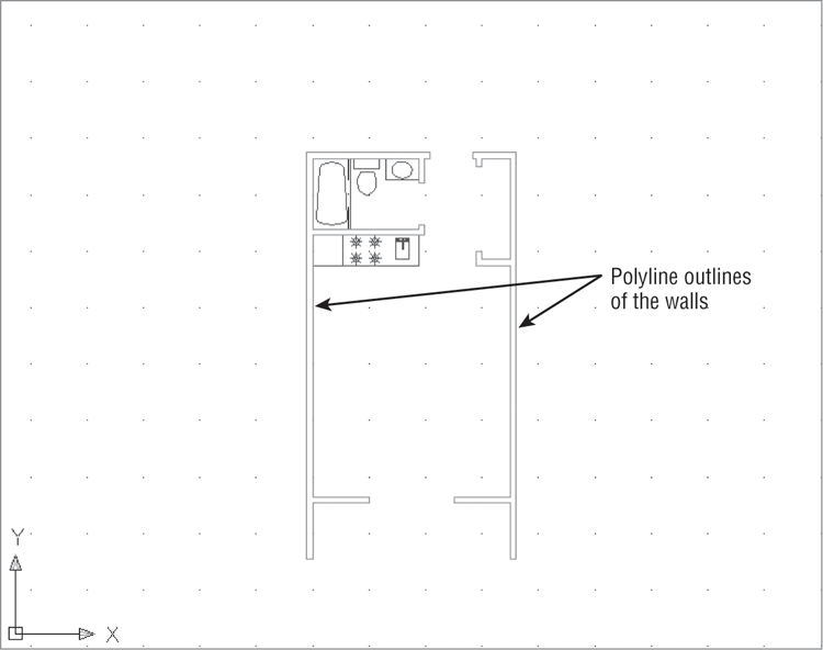
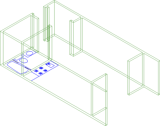
In the following set of exercises, you’ll turn the apartment room from previous chapters into a 3D model. We’ve created a version of the apartment floor plan that has a few additions to make things a little easier for you. Figure 21-19 shows the file you’ll use in the exercise. It’s the same floor plan with which you’ve been working in earlier chapters but with the addition of closed polylines outlining the walls.
Figure 21-19 The unit plan with closed polylines outlining the walls
The plan isn’t shaded as in the previous examples in this chapter. You can work in 3D in this display mode just as easily as in a shaded mode:
Figure 21-20 Selecting a view from the 3D Navigation drop-down list
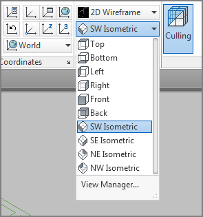
Figure 21-21 A 3D view of the unit plan
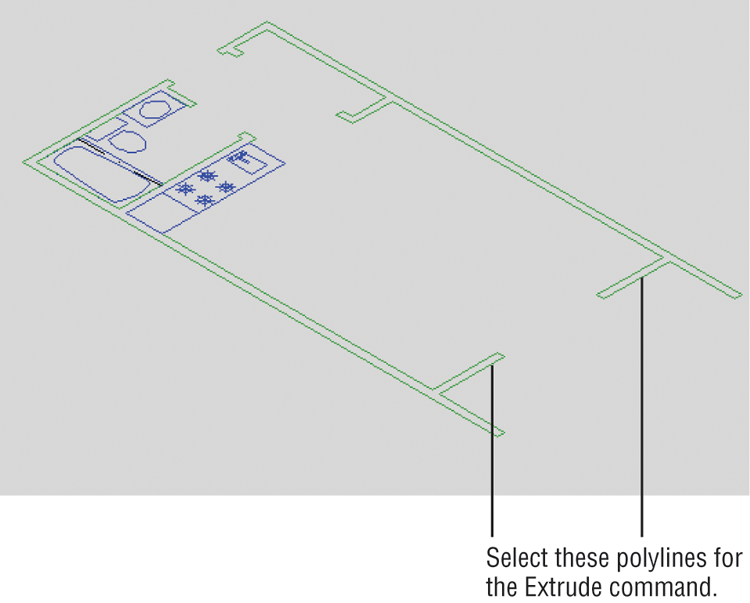
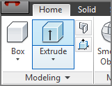
Figure 21-22 Selecting the Extrude tool from the Modeling panel
Unlike in the earlier exercise with the box, you can see through the walls because this is a Wireframe view. A Wireframe view shows the volume of a 3D object by displaying the lines representing the edges of surfaces. Later in this chapter, we’ll discuss how to make an object’s surfaces appear opaque as they do on the box earlier in this chapter.
Figure 21-23 The extruded walls
Next you’ll add door headers to define the wall openings:
Figure 21-24 Adding the door header to the opening at the balcony of the unit plan
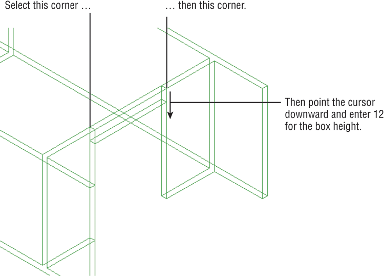
Figure 21-25 Adding the remaining door headers
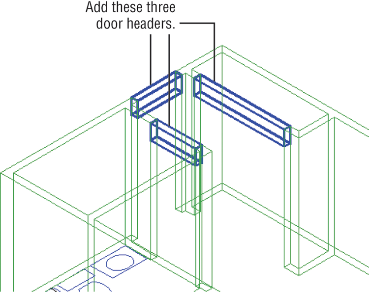
The walls and door headers give you a better sense of the space in the unit plan. To enhance the appearance of the 3D model further, you can join the walls and door headers so that they appear as seamless walls and openings:
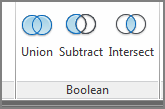
Figure 21-26 Select the Union tool.
Now the walls and headers appear as one seamless surface without any distracting joint lines. You can get a sense of the space of the unit plan. You’ll want to explore ways of viewing the unit in 3D, but before you do that, you need to know about one more 3D modeling feature: point filters.
Isolating Coordinates with Point Filters
AutoCAD offers a method for 3D point selection that can help you isolate the x-, y-, or z-coordinate of a location in 3D. Using point filters (described in the help files as “coordinate filters”), you can enter an X, Y, or Z value by picking a point on the screen and telling AutoCAD to use only the X, Y, or Z value of that point or any combination of those values. For example, suppose you want to start the corner of a 3D box at the x- and y-coordinates of the corner of the unit plan, but you want the Z location at 3′ instead of at ground level. You can use point or coordinate filters to select only the x- and y-coordinates of a point and then specify the z-coordinate as a separate value. The following exercise demonstrates how this works:
Figure 21-27 Constructing the rail using point filters
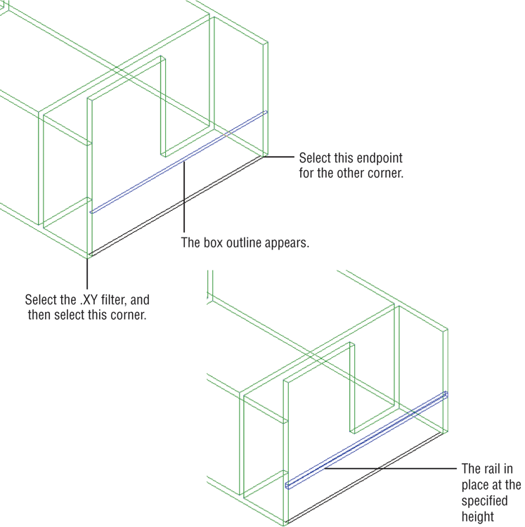
In step 4, you selected the corner of the unit, but the box didn’t appear right away. You had to enter a Z value in step 5 before the outline of the box appeared. Then, in step 6, you saw the box begin at the 36″ elevation. Using point filters allowed you to place the box accurately in the drawing even though there were no features that you could snap to directly.
Now that you’ve gotten most of the unit modeled in 3D, you’ll want to be able to look at it from different angles. Next you’ll see some of the tools available to control your views in 3D.
Moving Around Your Model
AutoCAD offers a number of tools to help you view your 3D model. You’ve already used one to get the current 3D view. Choosing Southwest Isometric from the View panel’s drop-down list displays an isometric view from a southwest direction. You may have noticed several other isometric view options in that list. The following sections introduce you to some of the ways you can move around in your 3D model.
Finding Isometric and Orthogonal Views
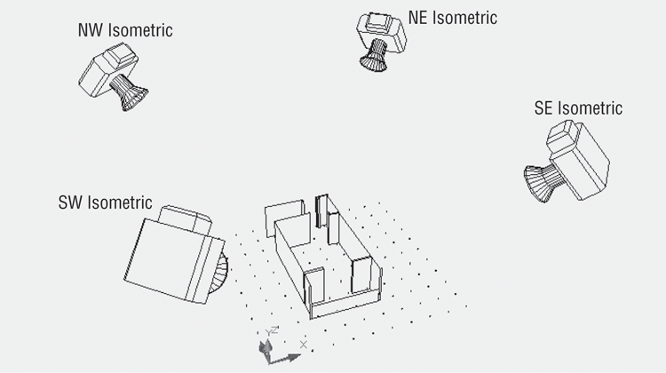
Figure 21-28 illustrates the isometric view options you saw earlier in the Home tab’s View panel drop-down list: Southeast Isometric, Southwest Isometric, Northeast Isometric, and Northwest Isometric. The cameras represent the different viewpoint locations. You can get an idea of their location in reference to the grid and UCS icon.
Figure 21-28 The isometric viewpoints for the four isometric views available from the Home tab’s View panel drop-down list
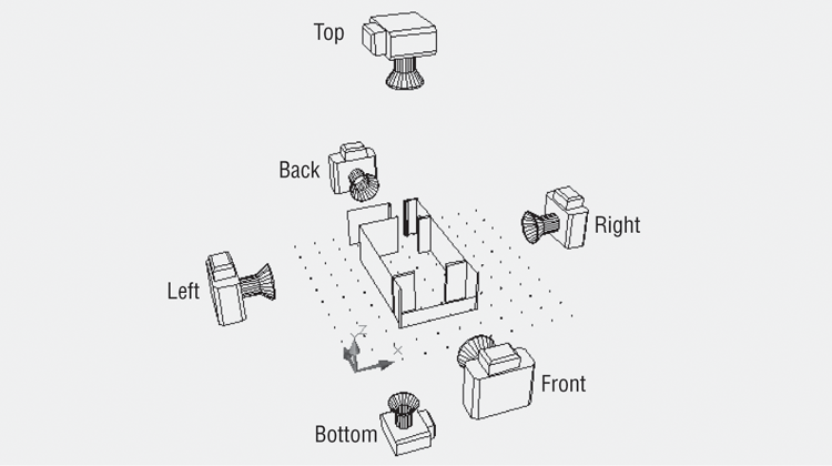
The Home tab’s View panel’s 3D Navigation drop-down list also offers another set of options: Top, Bottom, Left, Right, Front, and Back. These are orthogonal views that show the sides, top, and bottom of the model, as illustrated in Figure 21-29. In this figure, the cameras once again show the points of view.
Figure 21-29 This diagram shows the six viewpoints of the orthogonal view options on the View panel’s 3D Navigation drop-down list.
When you use any of the view options described here, AutoCAD attempts to display the extents of the drawing. You can then use the Pan and Zoom tools to adjust your view.
Rotating Freely Around Your Model
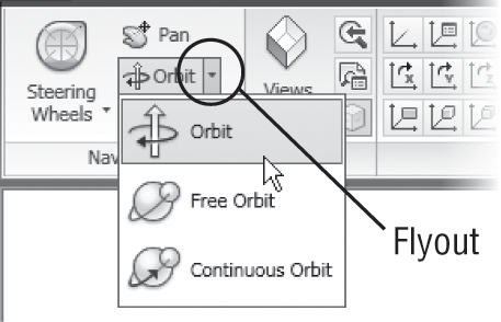
You may find the isometric and orthogonal views a bit restrictive. The Orbit tool lets you move around your model in real time. You can fine-tune your view by clicking and dragging the mouse using this tool. Try the following to see how it works:
If you have several objects in your model, you can select an object that you want to revolve around and then click the Orbit tool. It also helps to pan your view so that the object you select is in the center of the view.
When you’ve reached the view you want, right-click and choose Exit. You’re then ready to make more changes or use another tool.
Changing Your View Direction
One of the first tasks you’ll want to do with a model is to look at it from all angles. The ViewCube® tool is perfect for this purpose. The ViewCubeis a device that lets you select a view by using a sample cube. If it is not visible in your drawing, do the following:
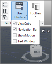
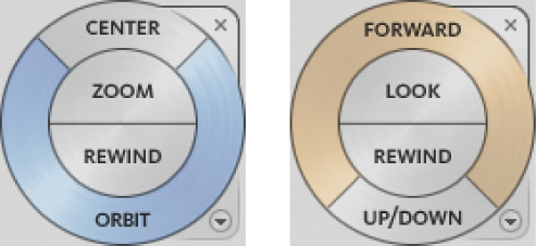
The following list explains what you can do with the ViewCube (see Figure 21-30):
Figure 21-30 The ViewCube and its options
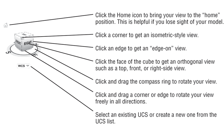
- Click the Home icon to bring your view to the “home” position. This is helpful if you lose sight of your model.
- You can get a top, front, right-side, or other orthogonal view just by clicking the word Top, Front, or Right on the ViewCube.
- Click a corner of the cube to get an isometric-style view, or click an edge to get an “edge-on” view.
- Click and drag the N, S, E, or W label to rotate the model in the XY plane.
- To rotate your view of the object in 3D freely, click and drag the cube.
- From the icon at the bottom, select an existing UCS or create a new one from the UCS list.
You can also change from a perspective view to a parallel projection view by right-clicking the cube and selecting Parallel Projection. To go from parallel projection to perspective, right-click and select Perspective or Perspective With Ortho Faces. The Perspective With Ortho Faces option works like the Perspective option except it will force a parallel projection view when you use the ViewCube to select a top, bottom, or side orthographic view.
When you are in a plan or top view, the ViewCube will look like a square, and when you hover your cursor over the cube, you’ll see two curved arrows to the upper right of the cube (see Figure 21-31).
Figure 21-31 The ViewCube top view
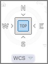
You can click on any of the visible corners to go to an isometric view or click the double-curved arrows to rotate the view 90 degrees. The four arrowheads that you see pointing toward the cube allow you to change to an orthographic view of any of the four sides.
Using SteeringWheels
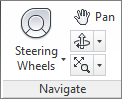
The ViewCube is great for looking at your model from different angles. But if your application requires you to be inside your model, you’ll want to know how to use the SteeringWheels® feature. The SteeringWheels feature collects a number of viewing tools in one interface. You can open SteeringWheels by clicking the SteeringWheels tool in the View tab’s Navigate panel (see Figure 21-32) or from the Navigation bar.
Figure 21-32 The SteeringWheels tool
You can also type Navswheel↵. When you do this, the SteeringWheels tool appears in the drawing area and moves with the cursor.
The SteeringWheels options are fairly self-explanatory. Just be aware that you need to use a click-and-drag motion to use them:
Figure 21-33 Placing the green sphere of the Center option
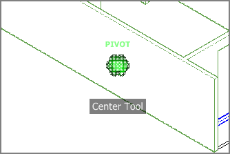
Figure 21-34 Using the Walk option
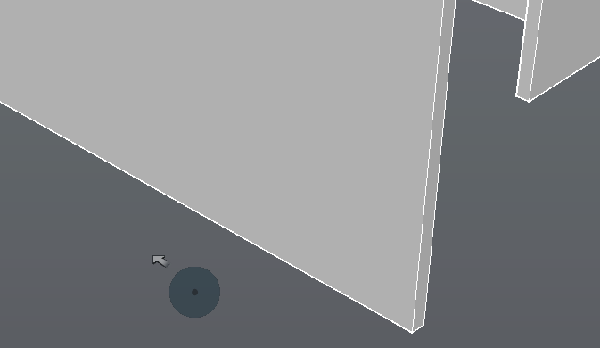
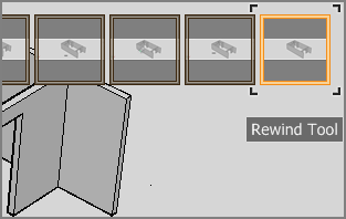
Figure 21-35 The frames of the Rewind tool
SteeringWheels offers a number of options in a right-click menu. This menu can also be opened by clicking the arrowhead in the lower-right corner of the wheel. Most of these right-click menu options are self-explanatory, but a few of them are worth a brief description.
If you click the Basic Wheels option in the SteeringWheels right-click menu, you’ll see Tour Building and View Object. Select the Tour Building Wheel option. Figure 21-36 shows these variations on the basic SteeringWheels wheel, and they offer a pared-down set of options for the two types of viewing options indicated by the name of the wheels.
Figure 21-36 Variations of the SteeringWheels wheel
You’ll also see mini versions available for the wheels from the SteeringWheels menu. The mini versions are much smaller, and they do not have labels indicating the options. Instead you see segmented circles, like a pie. Each segment of the circle is an option. Tool tips appear when you point at a segment, telling you what option that segment represents. Other than that, the mini versions work the same as the full-sized wheels.
The SteeringWheels feature takes a little practice, but once you’ve become familiar with it, you may find that you use it frequently when studying a 3D model. Just remember that a click-and-drag motion is required to use the tools effectively.
Changing Where You Are Looking
AutoCAD uses a camera analogy to help you set up views in your 3D model. With a camera, you have a camera location and a target, and you can fine-tune both in AutoCAD. AutoCAD also offers the Swivel tool to let you adjust your view orientation. Using the Swivel tool is like keeping the camera stationary while pointing in a different direction. While viewing your drawing in perspective mode, click Pan on the View tab’s Navigation bar, right-click in the drawing area, and select Other Navigation Modes ⇒ Swivel. (Remember that you need to right-click on the ViewCube and select Perspective for the perspective mode.)
At first the Swivel tool might seem just like the Pan tool. But in the 3D world, Pan actually moves both the camera and the target in unison. Using Pan is a bit like pointing a camera out the side of a moving car. If you don’t keep the view in the camera fixed on an object, you are panning across the scenery. Using the Swivel tool is like standing on the side of the road and turning the camera to take in a panoramic view.
To use the Swivel tool, do the following:
If you happen to lose your view entirely, you can use the Undo tool in the Quick Access toolbar to return to your previous view and start over.
Flying Through Your View
Another way to get around in your model is to use the Walk or Fly view options. If you’re familiar with computer games, this tool is for you. To get to these options, start the Pan tool as you did in the last exercise, and then right-click and select Other Navigation Modes ⇒ Fly. If you don’t see the Other Navigation Modes menu option, make sure that you are in a perspective view.
If you right-click while in this mode and click Display Instruction Window, a window will appear on the Communications Center. This message in the window tells you all you need to know about the Walk and Fly tools. You can use the arrow keys to move through your model. Click and drag the mouse to change the direction in which you’re looking.
If you press the F key, Walk changes to Fly mode. The main difference between Walk and Fly is that in Walk, both your position in the model and the point at which you’re looking move with the Up and Down arrow keys. Walk is a bit like Pan. When you’re in Fly mode, the arrow keys move you toward the center of your view, which is indicated by a crosshair.
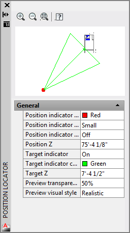
In addition to the crosshair, you’ll see a palette that shows your position in the model from a top-down view (see Figure 21-37).
You can use the palette to control your view by clicking and dragging the camera or the view target graphic. If you prefer, you can close the palette and continue to “walk” through your model. When you’re finished using Walk, right-click and choose Exit.
Figure 21-37 The Position Locator palette uses a top-down view.
Changing from Perspective to Parallel Projection
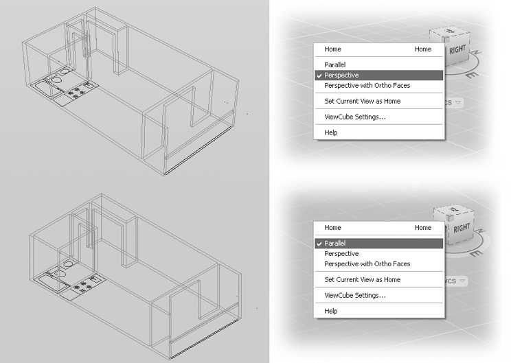
When you create a new drawing using the acad3D.dwt template, you’re automatically given a perspective view of the file. If you need a more schematic parallel projection style of view, you can get one from the ViewCube’s right-click menu (see Figure 21-38). You can return to a perspective view by using the same context menu shown in the figure.
Figure 21-38 The Perspective projection and Parallel projection tools
Getting a Visual Effect
Although 3D models are extremely useful in communicating your ideas to others, sometimes you find that the default appearance of your model isn’t exactly what you want. If you’re only in a schematic design stage, you may want your model to look more like a sketch instead of a finished product. Conversely, if you’re trying to sell someone on a concept, you may want a realistic look that includes materials and even special lighting.
AutoCAD provides a variety of tools to help you get a visual style, from a simple wireframe to a fully rendered image complete with chrome and wood. In the following sections, you’ll get a preview of what is available to control the appearance of your model. Later, in Chapter 23, you’ll get an in-depth look at rendering and camera tools that allow you to produce views from hand-sketched “napkin” designs to finished renderings.
Using Visual Styles
In the earlier tutorials in this chapter, you drew a box that appeared to be solid. When you then opened an existing file to extrude the unit plan into the third dimension, you worked in a Wireframe view. These views are known as visual styles in AutoCAD. You used the Shades Of Gray visual style when you drew the box. The unit plan used the default 2D Wireframe view that is used in the AutoCAD Classic style of drawing.
Sometimes, it helps to use a different visual style, depending on your task. For example, the 2D Wireframe view in your unit plan model can help you visualize and select things that are behind a solid. AutoCAD includes several shaded view options that can bring out various features of your model. Try the following exercises to explore some of the other visual styles:
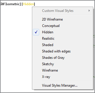
Figure 21-39 The Visual Styles drop-down
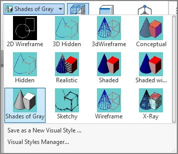
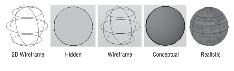
You may have noticed a few other Visual Styles options. Figure 21-40 shows a few of those options as they’re applied to a sphere. 2D Wireframe and Wireframe may appear the same, but Wireframe uses a perspective view and a background color, whereas 2D Wireframe uses a parallel projection view and no background color.
Figure 21-40 Visual styles applied to a sphere
Creating a Sketched Look with Visual Styles
You may notice blanks in the visual styles options in the View tab’s Visual Styles drop-down list. These spaces allow you to create custom visual styles. For practice, you’ll create a visual style similar to the existing Sketchy style so that you can learn how the rough look of that style was created. The following exercise will step you through the process:
Figure 21-41 The Visual Styles Manager
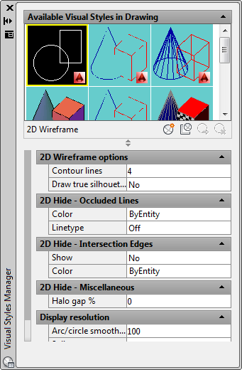
Figure 21-42 The Create New Visual Style dialog box
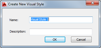
You’ve just created a new visual style. This new style uses the default settings that are similar to the Realistic visual style but without the Material Display option turned on. The material setting causes objects in your drawing to display any material assignments that have been given to objects. You’ll learn more about materials in Chapter 23.
Now that you have a new visual style, you can begin to customize it. But before you start your customization, make your new visual style the current one so that you can see the effects of your changes as you make them:
Figure 21-43 The 3D unit plan with the Sketch visual style
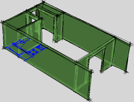
The 3D view has taken on a hand-drawn appearance. Notice that the lines overhang the corners in a typical architectural sketch style. This is the effect of the Line Extensions Edges option you used in step 3. The lines are made rough and broken by the Jitter Edges setting. You can control the amount of overhang and jitter in the Edge Modifiers group of the Visual Styles Manager to exaggerate or soften these effects.
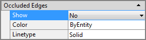
With your newly created Sketch visual style, the model looks like it’s transparent. You can make it appear opaque by turning off the Show option under the Occluded Edges group in the Visual Styles Manager (see Figure 21-44).
Figure 21-44 The Show option in the Occluded Edges group in the Visual Style Manager
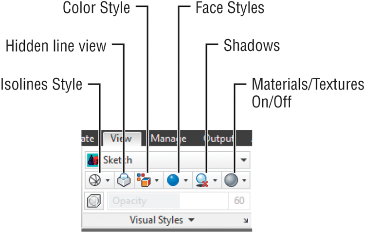
Finally, you can control some of the commonly used visual style properties using options in the View tab’s Visual Styles panel. This panel offers control over isolines, color, face style, shadows, and textures for the current visual style (see Figure 21-45).
Figure 21-45 Visual Styles options in the Visual Styles panel
In-Canvas Viewport Controls
Beginning in AutoCAD® 2012, controls are built into each viewport that allow you to quickly change between visual styles and model views without starting either command. These controls are found in the upper-left portion of the viewport. Clicking the view name will bring up a list of the available views to choose from. Likewise, clicking on the visual style will bring up a list of available visual styles. Clicking on either of them will instantly make the selected style or view current in that viewport.
Turning a 3D View into a 2D AutoCAD Drawing
Many architectural firms use AutoCAD 3D models to study their designs. After a specific part of a design is modeled and approved, they convert the model into 2D elevations, ready to plug into their elevation drawing.
If you need to convert your 3D models into 2D line drawings, you can use the Flatshot tool in the Home tab’s expanded Section panel.
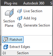
Set up your drawing view, and then click the Flatshot tool or enter Flatshot↵ at the command-line interface to open the Flatshot dialog box (see Figure 21-46).
Figure 21-46 The Flatshot dialog box
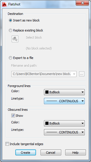
Select the options you want to use for the 2D line drawing, and then click Create. Depending on the options you select, you’ll be prompted to select an insertion point or indicate a location for an exported drawing file. The 2D line drawing will be placed on the plane of the current UCS, so if you are viewing your model in a 3D view but you are in the World UCS, the 2D line drawing will appear to be projected onto the XY plane.
Flatshot offers the ability to place the 2D version of your model in the current drawing as a block, to replace an existing block in the current drawing, or to save the 2D version as a DWG file. Table 21-1 describes the Flatshot options in more detail.
Table 21-1: Flatshot options
| Option | What it does |
| Destination | |
| Insert As New Block | Inserts the 2D view in the current drawing as a block. You’re prompted for an insertion point, a scale, and a rotation. |
| Replace Existing Block | Replaces an existing block with a block of the 2D view. You’re prompted to select an existing block. |
| Select Block | If Replace Existing Block is selected, lets you select a block to be replaced. A warning is shown if no block is selected. |
| Export To A File | Exports the 2D view as a drawing file. |
| Filename And Path | Displays the location for the export file. Click the Browse button to specify a location. |
| Foreground Lines | |
| Color | Sets the overall color for the 2D view. |
| Linetype | Sets the overall linetype for the 2D view. |
| Obscured Lines | |
| Show | Displays hidden lines. |
| Color | If Show is turned on, sets the color for hidden lines. |
| Linetype | If Show is turned on, sets the linetype for hidden lines. The Current Linetype Scale setting is used for linetypes other than continuous. |
| Include Tangential Edges | Displays edges for curved surfaces. |
- If you want to move a 3D solid using grips, you need to select the square grip at the bottom center of the solid. The other grips move only the feature associated with the grip, like a corner or an edge. Once that bottom grip is selected, you can switch to another grip as the base point for the move by doing the following: After selecting the base grip, right-click, select Base Point from the context menu, and click the grip you want to use.
- The Scale command will scale an object’s z-coordinate value as well as the standard x-coordinate and y-coordinate. Suppose you have an object with an elevation of 2 units. If you use the Scale command to enlarge that object by a factor of 4, the object will have a new elevation of 2 units times 4, or 8 units. If on the other hand that object has an elevation of 0, its elevation won’t change because 0 times 4 is still 0. You can use the 3dscale command to restrict the scaling of an object to a single plane.
- You can also use Mirror and Rotate (on the Modify panel) on 3D solid objects, but these commands don’t affect their z-coordinate values. You can specify z-coordinates for base and insertion points, so take care when using these commands with 3D models.
- Using the Move, Stretch, and Copy commands (on the Modify panel) with osnaps can produce unpredictable and unwanted results. As a rule, it’s best to use coordinate filters when selecting points with osnap overrides. For example, to move an object from the endpoint of one object to the endpoint of another on the same z-coordinate, invoke the .XY point filter at the Specify base point: and Specify second point: prompts before you issue the Endpoint override. Proceed to pick the endpoint of the object you want, and then enter the z-coordinate or pick any point to use the current default z-coordinate.
- When you create a block, it uses the currently active UCS to determine its own local coordinate system. When that block is later inserted, it orients its own coordinate system with the current UCS. (The UCS is discussed in more detail in Chapter 22.)
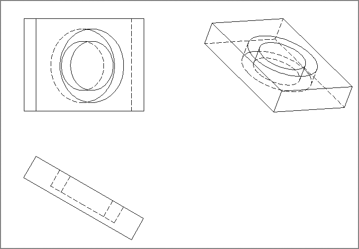
One useful feature of Flatshot is that it can create a 2D drawing that displays the hidden lines of a 3D mechanical drawing. Turn on the Show option, and then select a linetype such as Hidden for obscured lines to produce a 2D drawing like the one shown in Figure 21-47.
Figure 21-47 A sample of a 2D drawing generated from a 3D model using Flatshot. Note the dashed lines showing the hidden lines of the view.
Using the Point Cloud Feature
As you might guess from the name, a point cloud is a set of data points in a 3D coordinate system. They are often the product of 3D scanners, which are devices that can analyze and record the shape of real-world objects or environments. Point cloud data can be used to reproduce an object or environment as a digital model that can then be used for a video game, movie production, 3D model, or even as-built drawings.
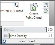
AutoCAD enables you to import raw point cloud data through a set of tools that can be found in the Insert tab’s Point Cloud panel (see Figure 21-48).
Figure 21-48 The Point Cloud panel in the Insert tab
AutoCAD can import point cloud data from several file types: FLS, FWS, LAS, XYB, XYZ, TXT, ASC, PTG, PTS, PTX, CLR, and CL3. You can also attach an indexed point cloud file through the External References palette just as you would a DWG, DWF, or other image file. AutoCAD can reference an ISD file, a PCG file, an RCP file, or an RCS file. The last two file types (Recap Project and RecapScan files) can be produced with the Autodesk ReCap program, a separate application that comes with AutoCAD (see the sidebar “Autodesk ReCap”).
Once the raw point cloud data has been imported, AutoCAD creates an ISD or PCG file from that data, indexes it, and displays it in your file. To import the data, use the Create Point Cloud tool in the Point Cloud panel. This tool can take some time to process a file, so indexing is performed in the background. This enables you to continue to work while a file is being indexed.
The indexing icon appears in the status bar to remind you that a point cloud is being indexed. If for some reason you need to cancel the indexing, you can right-click the icon and select Cancel Indexing.
Once AutoCAD has produced an ISD or PCG file from the indexed data, these files can then be attached to a drawing file using the Attach tool in the Point Cloud panel, or through the Xref Manager. Selecting an attached point cloud displays a bounding box around the data and activates the contextual Cloud Edit Ribbon tab. This tab provides a set of tools that you can use to manipulate your point cloud by clipping it (similar to the Clip tool), changing the point density, adjusting the color display of the point cloud, or running analysis tools.
Because point clouds can consume a great deal of memory, you can use the Density slider in the expanded Point Cloud panel to control the density of the point cloud or in the Cloud Edit Ribbon tab. The lower the density, the less impact the point cloud will have on performance. You can also control the real-time density of the point cloud while zooming or panning in your file. The lower the real-time density, the quicker AutoCAD can process the point cloud while you zoom or pan.
Once you have the point cloud attached to a drawing, you can use the points to help guide you in building a 3D model. You can use the Node osnap to snap to the individual points in the point cloud. The referenced Point Cloud is selectable. When you do select it, a Contextual Ribbon tab will appear. This tab has several tools that will help you display your point cloud. There are slider bars to increase or decrease the density of the points (how many are currently being displayed). You can change the color of the points or use any color data your scanning device may have gathered. There are also clipping tools to help speed up your file by reducing the number of points to process. This clipping feature can also help control what is being displayed in your file.