Chapter 24
Editing and Visualizing 3D Solids
In the previous 3D chapters, you spent some time becoming familiar with the AutoCAD® software’s 3D modeling features. In this chapter, you’ll focus on 3D solids and how they’re created and edited. You’ll also learn how you can use some special visualization tools to show your 3D solid in a variety of ways.
You’ll create a fictitious mechanical part to explore some of the ways you can shape 3D solids. This will also give you a chance to see how you can turn your 3D model into a standard 2D mechanical drawing. In addition, you’ll learn about the 3D solid-editing tools that are available through the Solid Editing Ribbon panel.
In this chapter, you will learn to:
- Understand solid modeling
- Create solid forms
- Create complex solids
- Edit solids
- Streamline the 2D drawing process
- Visualize solids
Understanding Solid Modeling
Solid modeling is a way of defining 3D objects as solid forms. When you create a 3D model by using solid modeling, you start with the basic forms of your model—boxes, cones, and cylinders, for example. These basic solids are called primitives. Then, using more of these primitives, you begin to add to or subtract from your basic forms.
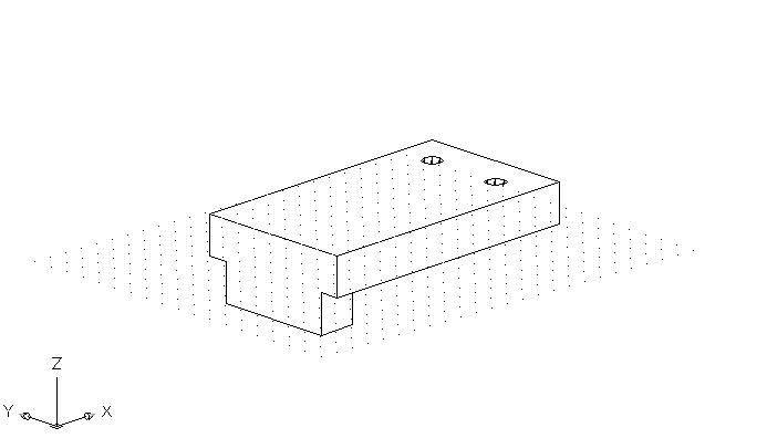
For example, to create a model of a tube you first create two solid cylinders, one smaller in diameter than the other. You then align the two cylinders so that they’re concentric and tell AutoCAD to subtract the smaller cylinder from the larger one. The larger of the two cylinders becomes a tube whose inside diameter is that of the smaller cylinder, as shown in Figure 24-1. Several primitives are available for modeling solids in AutoCAD (see Figure 24-2).
Figure 24-1 Creating a tube by using solid modeling
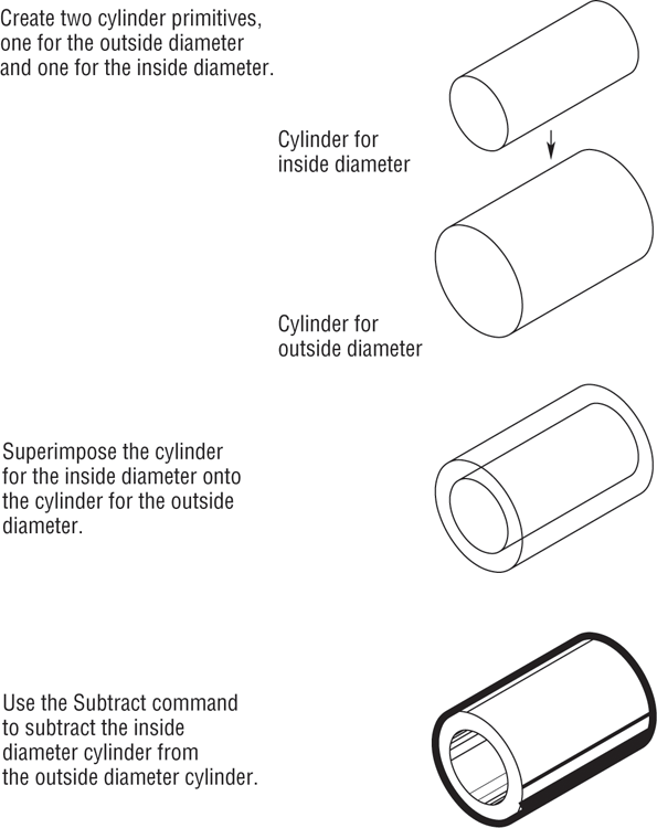
Figure 24-2 The solid primitives
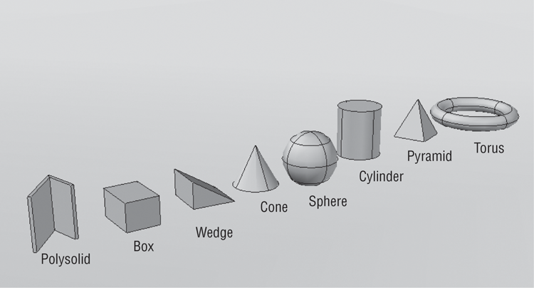
You can join these shapes—polysolid, box, wedge, cone, sphere, cylinder, pyramid, and donut (or torus)—in one of four ways to produce secondary shapes. The first three, demonstrated in Figure 24-3 using a cube and a cylinder as examples, are called Boolean operations. (The name comes from the nineteenth-century mathematician George Boole.)
Figure 24-3 The intersection, subtraction, and union of a cube and a cylinder
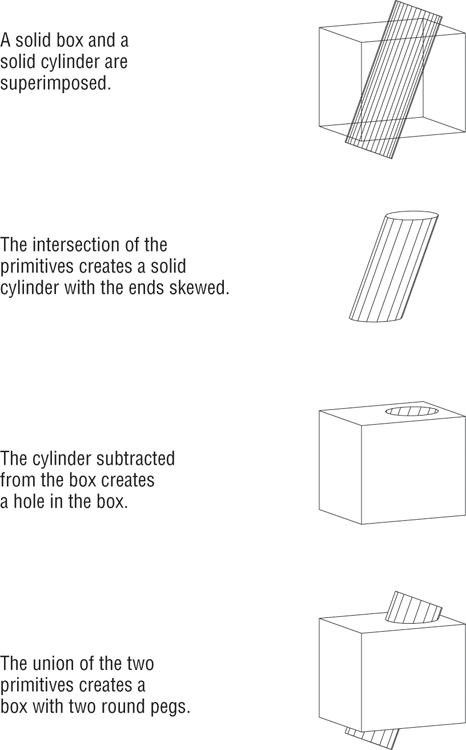
The three Boolean operations are as follows:
The fourth option, Interfere, lets you find exactly where two or more solids coincide in space—similar to the results of a union. The main difference between interference and union is that interference enables you to keep the original solid shapes, whereas union discards the original solids, leaving only their combined form. Interfere creates a temporary 3D solid of the coincident space. You can close the command or have AutoCAD create a solid based on the shape created. The selected objects will remain unchanged.
Joined primitives are called composite solids. You can join primitives to primitives, composite solids to primitives, and composite solids to other composite solids.
Now let’s look at how you can use these concepts to create models in AutoCAD.
Creating Solid Forms
In the following sections, you’ll begin to draw the object shown later in the chapter in Figure 24-18. In the process, you’ll explore the creation of solid models by creating primitives and then setting up special relationships between them.
Primitives are the basic building blocks of solid modeling. At first, it may seem limiting to have only eight primitives with which to work, but consider the varied forms you can create with just a few two-dimensional objects. Let’s begin by creating the basic mass of your steel bracket.
First, prepare your drawing for the exercise:
Joining Primitives
In this section, you’ll merge the two box objects. First you’ll move the new box into place. Then you’ll join the two boxes to form a single solid:
Figure 24-4 Moving the smaller box
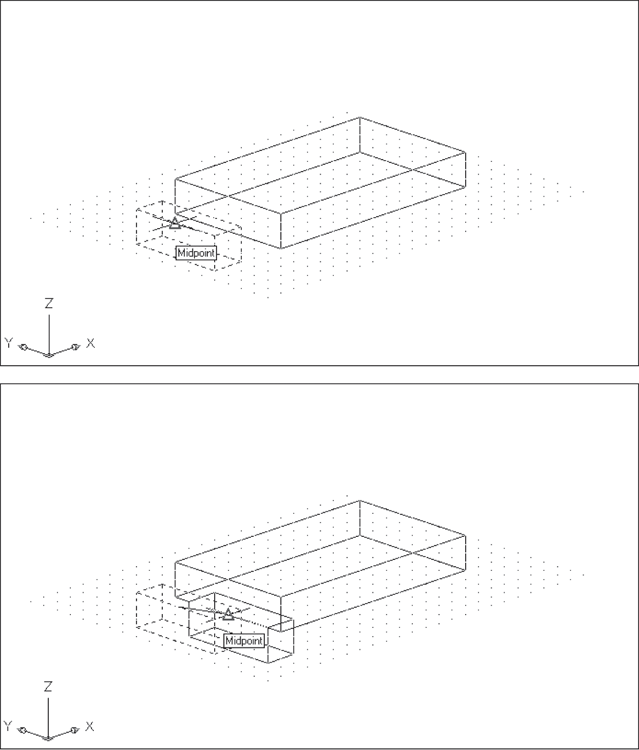
Figure 24-5 The two boxes joined
As you can see in Figure 24-5, the form has joined to appear as one object. It also acts like one object when you select it. You now have a composite solid made up of two box primitives.
Cutting Portions Out of a Solid
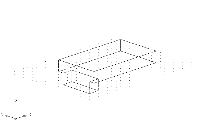
Now let’s place some holes in the bracket. In this next exercise, you’ll discover how to create negative forms to cut portions out of a solid:
Figure 24-6 The cylinders appear when the Cylinder layer is turned on.
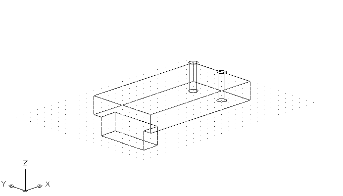
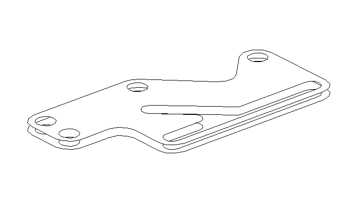
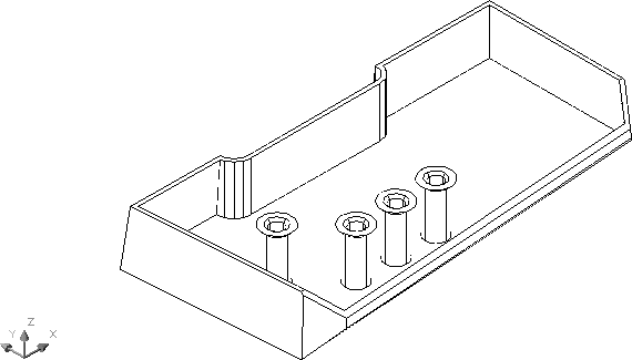
Figure 24-7 The bracket so far, with hidden lines removed
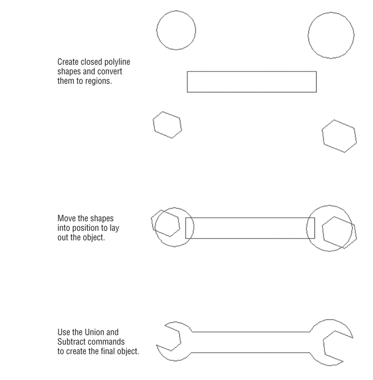
- Regions act like surfaces; when you remove hidden lines, objects behind the regions are hidden.
- You can explode regions to edit them. However, exploding a region causes the region to lose its surface-like quality, and objects no longer hide behind its surface(s).
- You can Ctrl+click the edge of a region to edit the region’s shape.
- You can use the regional model to create complex 2D surfaces for use in 3D surface modeling, as in this image:
As you learned in the earlier chapters in Part 4, Wireframe views, such as the one in the previous exercise, are somewhat difficult to decipher. Until you use the Hidden visual style (step 5) or the Hide command, you can’t be sure that the subtracted cylinders are in fact holes. Using the Hide command frequently will help you keep track of what’s going on with your solid model.
You may also have noticed in step 4 that, even though the cylinders were taller than the opening they created, they worked fine to remove part of the rectangular solid. The cylinders were 1.5 units tall, not 1 unit, which is the thickness of the bracket. Having drawn the cylinders taller than needed, you saw that when AutoCAD performed the subtraction, it ignored the portion of the cylinders that didn’t affect the bracket. AutoCAD always discards the portion of a primitive that isn’t used in a subtract operation.
Creating Complex Solids
As you learned earlier, you can convert a polyline into a solid by using the Extrude tool in the Modeling panel. This process lets you create more complex shapes than the built-in primitives. In addition to the simple straight extrusion you’ve already tried, you can extrude shapes into curved paths or you can taper an extrusion.
Tapering an Extrusion
Let’s look at how you can taper an extrusion to create a fairly complex solid with little effort:
Figure 24-8 The extruded polyline
In step 5, you can indicate a taper for the extrusion. Specify a taper in terms of degrees from the z-axis, or enter a negative value to taper the extrusion outward. You can also press ↵ to accept the default of 0° to extrude the polyline without a taper.
Current wire frame density: ISOLINES=4Sweeping a Shape on a Curved Path
As you’ll see in the following exercise, the Sweep command lets you extrude virtually any polyline shape along a path defined by a polyline, an arc, or a 3D polyline. At this point, you’ve created the components needed to do the extrusion. Next you’ll finish the extruded shape:
Figure 24-9 Hidden-line view showing parts of the drawing you’ll use to create a curved extrusion
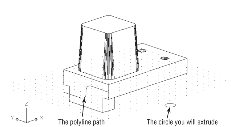
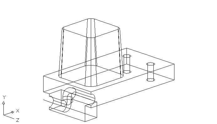
Figure 24-10 The solid after subtracting the curve
In this exercise, you used a curved polyline for the extrusion path, but you can use any type of 2D or 3D polyline, as well as a line or arc, for an extrusion path.
Revolving a Polyline
When your goal is to draw a circular object, you can use the Revolve command on the Modeling panel to create a solid that is revolved, or swept in a circular path. Think of Revolve’s action as being similar to a lathe that lets you carve a shape from an object on a spinning shaft. In this case, the object is a polyline and, rather than carve it, you define the profile and then revolve the profile around an axis.
In the following exercise, you’ll draw a solid that will form a slot in the tapered solid. We’ve already created a 2D polyline that is the profile of the slot. You’ll simply use cut and paste to bring the polyline into the bracket drawing:
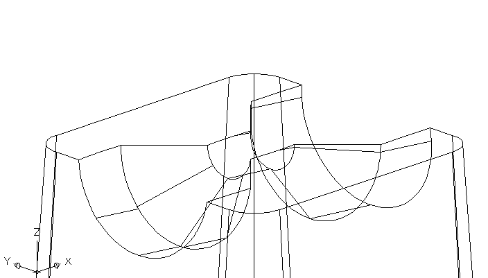
Figure 24-11 An enlarged view of the top of the tapered box and pasted polyline
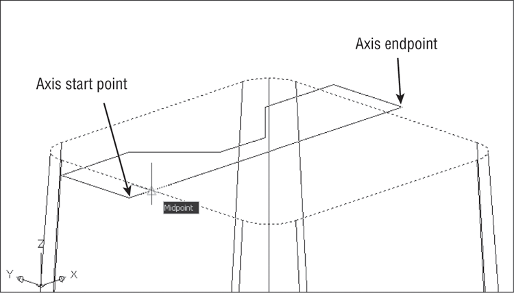
Specify axis start point or define axis by [Object/X/Y/Z] <Object>:Figure 24-12 The revolved polyline
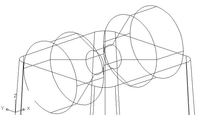
You just created a revolved solid that will be subtracted from the tapered box to form a slot in the bracket. However, before you subtract it, you need to make a slight change in the orientation of the revolved solid:
Current positive angle in UCS:  ANGDIR=counterclockwise  ANGBASE=0
Select objects:Figure 24-13 Selecting the points to rotate the revolved solid in 3D space
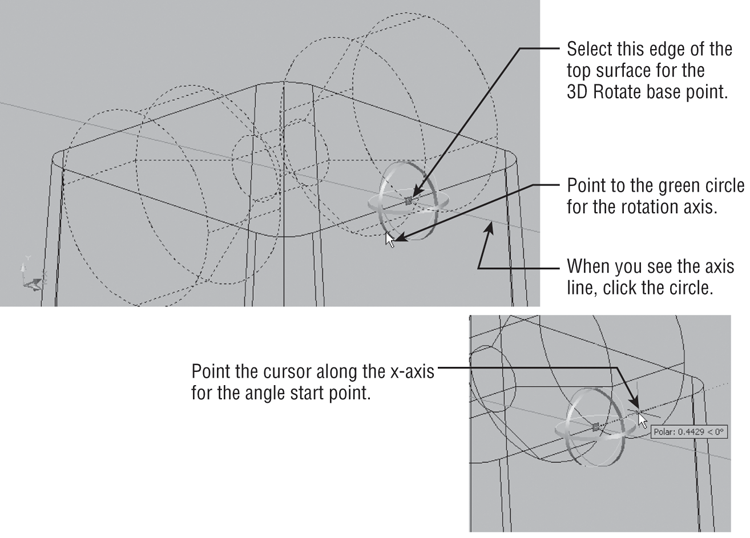
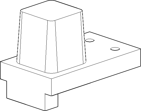
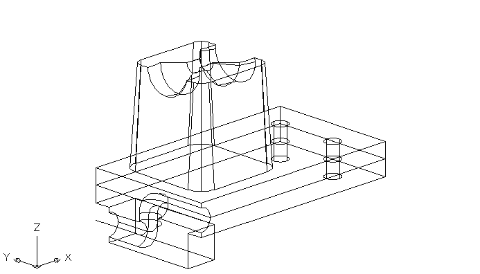
Figure 24-14 The composite solid
Editing Solids
Basic solid forms are fairly easy to create. Refining those forms requires some special tools. In the following sections, you’ll learn how to use familiar 2D editing tools, as well as some new tools, to edit a solid. You’ll also be shown the Slice tool, which lets you cut a solid into two pieces.
Splitting a Solid into Two Pieces
One of the more common solid-editing tools you’ll use is the Slice tool. As you may guess from its name, Slice enables you to cut a solid into two pieces. The following exercise demonstrates how it works:
Specify start point of slicing plane or
[planar Object/Surface/Zaxis/View/XY/YZ/ZX/
3points] <3points>:Figure 24-15 The solid sliced through the base
In step 4, you saw a number of options for the Slice command. You may want to take note of those options for future reference. Table 24-1 provides a list of the options and their purposes.
Table 24-1: Slice command options
| Option | Purpose |
| planar Object | Lets you select an object to define the slice plane. |
| Surface | Lets you select a surface object to define the shape of a slice. |
| Zaxis | Lets you select two points defining the z-axis of the slice plane. The two points you pick are perpendicular to the slice plane. |
| View | Generates a slice plane that is perpendicular to your current view. You’re prompted for the coordinate through which the slice plane must pass—usually a point on the object. |
| XY/YZ/ZX | Pick one of these to determine the slice plane based on the x-, y-, or z-axis. You’re prompted to pick a point through which the slice plane must pass. |
| 3points | The default setting; lets you select three points defining the slice plane. Normally, you pick points on the solid. |
Rounding Corners with the Fillet Tool
Your bracket has a few sharp corners that you may want to round in order to give it a more realistic appearance. You can use the Modify panel’s Fillet and Chamfer tools to add these rounded corners to your solid model:
Figure 24-16 Filleting solids
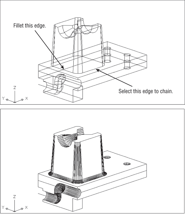
As you saw in step 4, Fillet acts a bit differently when you use it on solids. The Chain option lets you select a set of edges instead of just two adjoining objects.
Chamfering Corners with the Chamfer Tool
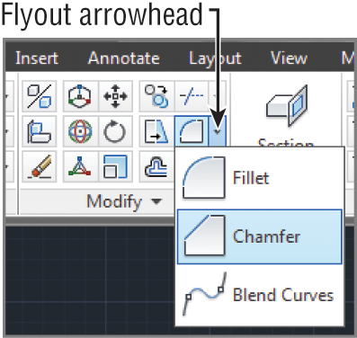
Now let’s try chamfering a corner. To practice using Chamfer, you’ll add a countersink to the cylindrical hole you created in the first solid:
Figure 24-17 Click the Chamfer tool.
Select first line or
[Undo/Polyline/Distance/Angle/Trim/mEthod/Multiple]:Figure 24-18 Picking the edge to chamfer
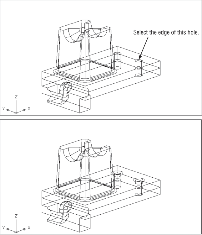
Figure 24-19 The chamfered edges
The Loop option in step 7 lets you chamfer the entire circumference of an object. You don’t need to use it here because the edge forms a circle. The Loop option is used when you have a rectangular or other polygonal edge you want to chamfer.
Using the Solid-Editing Tools
You’ve added some refinements to the Bracket model by using standard AutoCAD editing tools. There is a set of tools that is specifically geared toward editing solids. You already used the Union and Subtract tools found in the Solid Editing panel. In the following sections, you’ll explore some of the other tools in that panel.
You don’t have to perform the following exercises, but reviewing them will show you what’s available. When you’re more comfortable working in 3D, you may want to come back and experiment with the file called solidedit.dwg shown in the figures in the following sections.
Finding Tools in the Solid Editing Panel
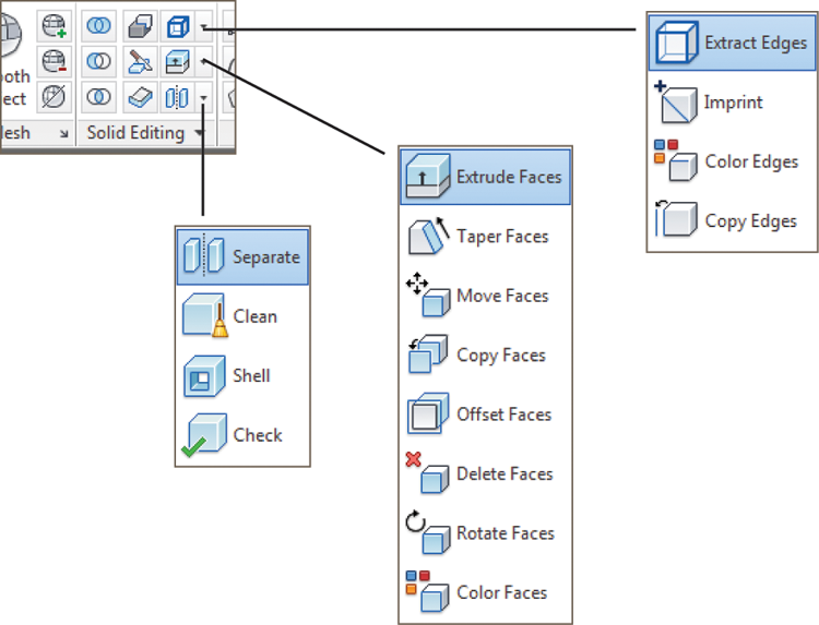
Many of the tools in the Solid Editing panel are in flyouts. This makes it a bit difficult to describe their location because the default tool changes depending on the last flyout tool that was selected. To help you easily find the tools described in these sections, Figure 24-20 shows the flyouts in their open position with each tool labeled. You can use this figure for reference when you are ready to use a tool.
Figure 24-20 The flyouts in the Home tab’s Solid Editing panel
Moving a Surface
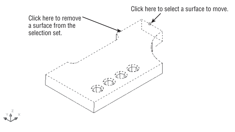
You can move any flat surface of a 3D solid using the Move Faces tool from the Faces flyout on the Solid Editing panel. When you click this tool, you’re prompted to select faces. Because you can select only the edge of two joining faces, you must select an edge and then use the Remove option to remove one of the two selected faces from the selection set (see Figure 24-21). Once you’ve made your selection, press ↵. You can then specify a distance for the move.
Figure 24-21 To select the vertical surface to the far right of the model, click the edge and then use the Remove option to remove the top surface from the selection.
After you’ve selected the surface you want to move, the Move Faces tool acts just like the Move command: You select a base point and a displacement. Notice how the curved side of the model extends its curve to meet the new location of the surface. This shows you that AutoCAD attempts to maintain the geometry of the model when you make changes to the faces.
Move Faces also lets you move entire features, such as the hole in the model. In Figure 24-22, one of the holes has been moved so that it’s no longer in line with the other three. This was done by selecting the countersink and the hole while using the Move Faces tool.
Figure 24-22 Selecting a surface to offset
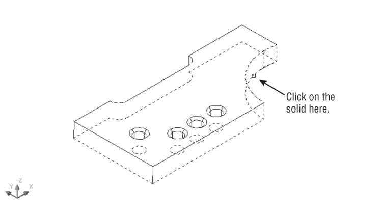
If a solid’s History setting is set to record, you can Ctrl+click on its surface to expose the surface’s grip. You can then use the grip at the center of the surface to move the surface.
Offsetting a Surface
Suppose you want to decrease the radius of the arc in the right corner of the model and you also want to thicken the model by the same amount as the decrease in the arc radius. To do this, you can use the Offset Faces tool. The Offset Faces tool and the Offset command you used earlier in this book perform similar functions. The difference is that the Offset Faces tool in the Faces flyout on the Solid Editing panel affects 3D solids.
When you select the Offset Faces tool from the Faces flyout on the Solid Editing panel, you’re prompted to select faces. As with the Move tool, you must select an edge that will select two faces. If you want to offset only one face, you must use the Remove option to remove one of the faces. In Figure 24-22, an edge is selected. Figure 24-23 shows the effect of the Offset Faces tool when both faces are offset.
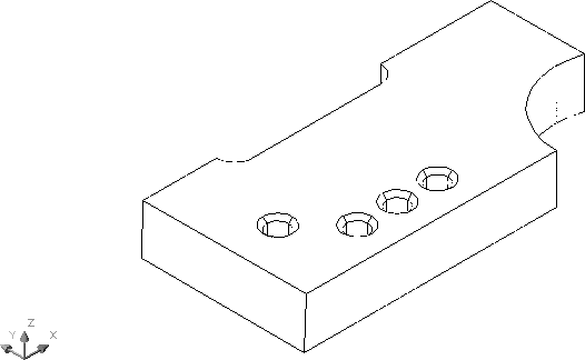
Figure 24-23 The model after offsetting the curved and bottom surfaces
Deleting a Surface
Now suppose you’ve decided to eliminate the curved part of the model. You can delete a surface by using the Delete Faces tool. Once again, you’re prompted to select faces. Typically, you’ll want to delete only one face, such as the curved surface in the example model. You use the Remove option to remove the adjoining face that you don’t want to delete before finishing your selection of faces to remove.
When you attempt to delete surfaces, keep in mind that the surface you delete must be recoverable by other surfaces in the model. For example, you can’t remove the top surface of a cube, expecting it to turn into a pyramid. That would require the sides to change their orientation, which isn’t allowed in this operation. You can, on the other hand, remove the top of a box with tapered sides. Then, when you remove the top, the sides converge to form a pyramid.
Rotating a Surface
All the surfaces of the model are parallel or perpendicular to each other. Imagine that your design requires two sides to be at an angle. You can change the angle of a surface by using the Rotate Faces tool.
As with the prior solid-editing tools, you’re prompted to select faces. You must then specify an axis of rotation. You can either select a point or use the default of selecting two points to define an axis of rotation, as shown in Figure 24-24. Once the axis is determined, you can specify a rotation angle. Figure 24-25 shows the result of rotating the two front-facing surfaces 4°.
Figure 24-24 Defining the axis of rotation
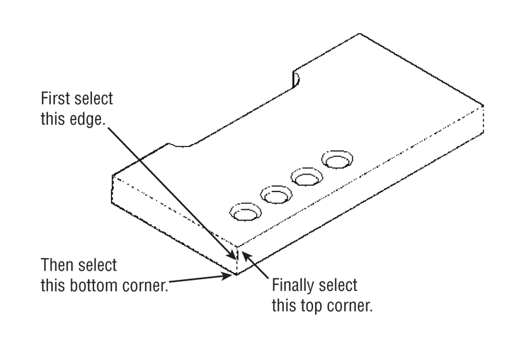
Figure 24-25 The model after rotating two surfaces
Tapering a Surface
In an earlier exercise, you saw how to create a new tapered solid by using the Extrude command. But what if you want to taper an existing solid? Here’s what you can do.
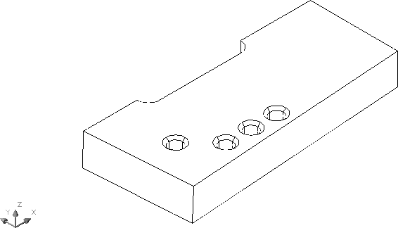
The Taper Faces tool from the Faces flyout on the Solid Editing panel prompts you to select faces. You can select faces, as described for the previously discussed solid-editing tools, using the Remove or Add option (see Figure 24-26). Press ↵ when you finish your selection, and then indicate the axis from which the taper is to occur. In the model example in Figure 24-26, select two corners defining a vertical axis. Finally, enter the taper angle. Figure 24-27 shows the model tapered at a 4° angle.
Figure 24-26 Selecting the surfaces to taper and indicating the direction of the taper
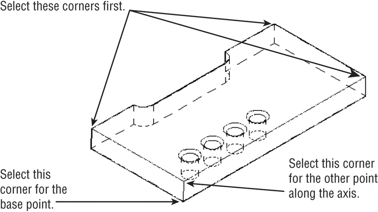
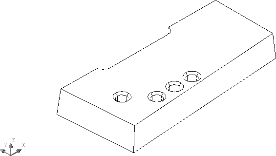
Figure 24-27 The model after tapering the sides
Extruding a Surface
You’ve used the Extrude tool to create two of the solids in the Bracket model. The Extrude tool requires a closed polyline as a basis for the extrusion. As an alternative, the Solid Editing panel offers the Extrude Faces tool, which extrudes a surface of an existing solid.
When you select the Extrude Faces tool from the Faces flyout on the Solid Editing panel or type Solidedit↵F↵E↵, you see the Select faces or [Undo/Remove]: prompt. Select an edge or a set of edges or use the Remove or Add option to select the faces you want to extrude. Press ↵ when you’ve finished your selection, and then specify a height and taper angle. Figure 24-28 shows the sample model with the front surface extruded and tapered at a 45° angle. You can extrude multiple surfaces simultaneously if you need to by selecting them.
Figure 24-28 The model with a surface extruded and tapered
Aside from those features, the Extrude Faces tool works just like the Extrude command.
Turning a Solid into a Shell
In many situations, you’ll want your 3D model to be a hollow mass rather than a solid mass. The Shell tool lets you convert a solid into a shell.
When you select the Shell tool from the Separate/Clean/Shell/Check flyout on the Solid Editing panel or type Solidedit↵B↵S↵, you’re prompted to select a 3D solid. You’re then prompted to remove faces. At this point, you can select an edge of the solid to indicate the surface you want removed. The surface you select is completely removed from the model, exposing the interior of the shell. For example, if you select the front edge of the sample model shown in Figure 24-29, the top and front surfaces are removed from the model, revealing the interior of the solid, as shown in Figure 24-30. After selecting the surfaces to remove, you can enter a shell offset distance.
The shell thickness is added to the outside surface of the solid. When you’re constructing your solid with the intention of creating a shell, you need to take this into account.
Figure 24-29 Selecting the edge to be removed
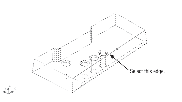
Figure 24-30 The solid model after using the Shell tool
Copying Faces and Edges
At times, you may want to create a copy of a surface of a solid to analyze its area or to produce another part that mates to that surface. The Copy Faces tool (found in the Extrude Faces flyout) creates a copy of any surface on your model. The copy it produces is a type of object called a region.
The copies of the surfaces are opaque and can hide objects behind them when you perform a hidden-line removal (type Hide↵).
Another tool that is similar to Copy Faces is Copy Edges (found in the Extract Edges flyout). Instead of selecting surfaces as in the Copy Faces tool, you select all the edges you want to copy. The result is a series of simple lines representing the edges of your model. This tool can be useful if you want to convert a solid into a set of 3D faces. The Copy Edges tool creates a framework onto which you can add 3D faces.
Adding Surface Features
If you need to add a feature to a flat surface, you can do so with the Imprint tool. An added surface feature can then be colored using the Color Faces tool or extruded using the Presspull tool. This feature is a little more complicated than some of the other solid-editing tools, so you may want to try the following exercise to see firsthand how it works.
You’ll start by inserting an object that will be the source of the imprint. You’ll then imprint the main solid model with the object’s profile:
You now have an outline of the intersection between the two solids imprinted on the top surface of your model. The imprint is really a set of edges that have been added to the surface of the solid. To help the imprint stand out, try the following steps to change its color:
If you want to remove an imprint from a surface, Ctrl+click the imprint and press the Delete key.
Separating a Divided Solid
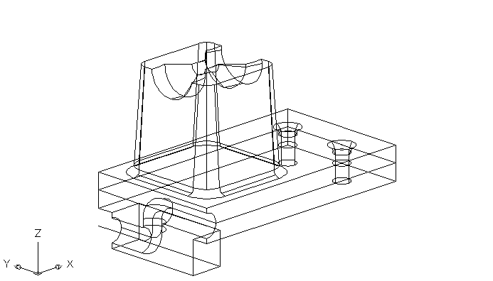
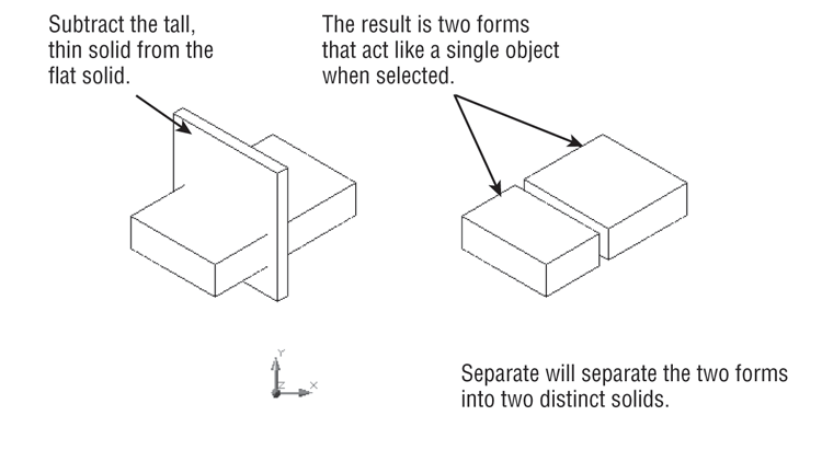
While editing solids, you can end up with two separate solid forms that were created from one solid, as shown in Figure 24-31. Even though the two solids appear separated, they act like a single object. In these situations, AutoCAD offers the Separate tool from the Separate/Clean/Shell/Check flyout on the Solid Editing panel. To use it, click the Separate tool or type Solidedit↵B↵P↵ and select the solid that has been separated into two forms.
Figure 24-31 is included in the sample files under the name Separate example.dwg. You can try the Separate tool in this file on your own.
Figure 24-31 When the tall, thin solid is subtracted from the larger solid, the result is two separate forms, yet they still behave as a single object.
Enter a solids editing option [Face/Edge/Body/Undo/eXit] <eXit>:[Extrude/Move/Rotate/Offset/Taper/Delete/Copy/coLor/mAterial/Undo/eXit] <eXit>:Enter an edge editing option [Copy/coLor/Undo/eXit] <eXit>:[Imprint/seParate solids/Shell/cLean/Check/Undo/eXit] <eXit>:Through some simple examples, you’ve seen how each of the solid-editing tools works. You aren’t limited to using these tools in the way they were demonstrated in this chapter, and this book can’t anticipate every situation you might encounter as you create solid models. These examples are intended as an introduction to these tools, so feel free to experiment with them. You can always use the Undo option to backtrack in case you don’t get the results you expect.
This concludes your tour of the Solid Editing panel. Next you’ll learn how to use 3D solid models to generate 2D working drawings quickly.
Streamlining the 2D Drawing Process
Using solids to model a part—such as with the bracket and Solidedit examples in this chapter—may seem a bit exotic, but there are definite advantages to modeling in 3D, even if you only want to show the part in 2D as a page in a set of manufacturing specs.
The exercises in the following sections show you how to generate a typical mechanical drawing from your 3D model quickly by using Paper Space and the Solid Editing panel. You’ll also examine techniques for dimensioning and including hidden lines.
Drawing Standard Top, Front, and Right-Side Views
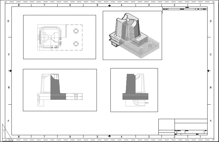
One of the more common types of mechanical drawings is the orthogonal projection. This style of drawing shows separate top, front, and right-side views of an object. Sometimes a 3D image is added for clarity. You can derive such a drawing in a few minutes using the Flatshot tool described in Chapter 21, “Creating 3D Drawings” (see “Turning a 3D View into a 2D AutoCAD Drawing” in that chapter).
With Flatshot, you can generate the standard top, front, and right-side orthogonal projection views, which you can further enhance with dimensions, hatch patterns, and other 2D drawing features. Follow these steps:
Figure 24-32 The 3D Navigation drop-down list

Figure 24-33 The Flatshot dialog box
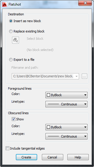
If you select Insert As New Block in the Flatshot dialog box, you’re prompted to select an insertion point to insert the block that is the 2D orthogonal view of your model. By default, the view is placed in the same plane as your current view as shown in Figure 24-34. Once you’ve created all your views, you can move them to a different location in your drawing so that you can create a set of layout views to your 2D orthogonal views, as shown in Figure 24-35. You can also place the orthogonal view blocks on a separate layer and then, for each layout viewport, freeze the layer of the 3D model so that only the 2D views are displayed.
Figure 24-34 The 2D orthogonal views shown in relation to the 3D model

Figure 24-35 You can use a layout to arrange a set of views created by Flatshot. Dimensions, notes, and a title block can be added to complete the layout.
If your model changes and you need to update the orthogonal views, you can repeat the steps listed here. However, instead of selecting Insert As New Block in the Flatshot dialog box, select Replace Existing Block to update the original orthogonal view blocks. If you want, you can include an isometric view to help communicate your design more clearly.
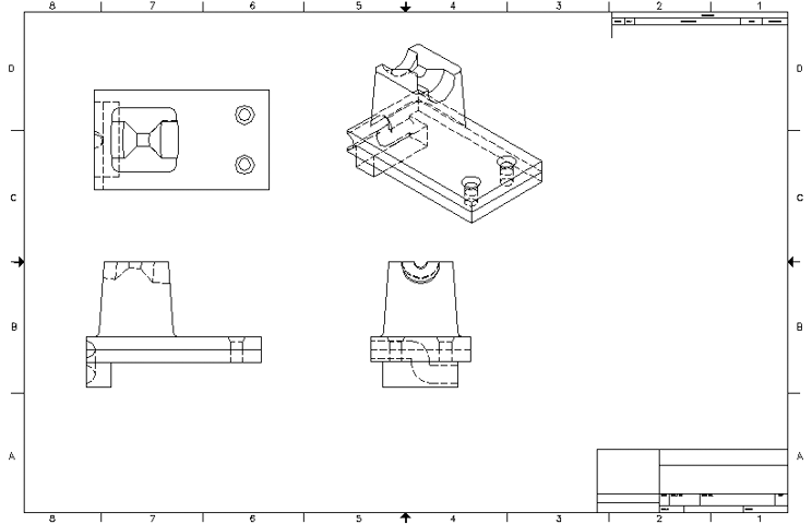
Creating 2D Drawings with the Base View Command
You saw how 2D views of a 3D model can be made using the Flatshot command. The Base View command also creates 2D views, but in a different way. Follow these steps for a demonstration:
Figure 24-36 The Base View command in the Layout tab of the Ribbon
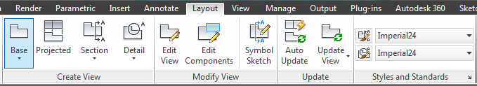
Figure 24-37 After you place the parent base view, this menu displays the options you can set.
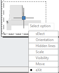
Figure 24-38 The Base View command can quickly create projection views of your 3D model.

You can now perform basic manipulations on the inserted views. Specifically, you can add or remove views at any time. Any view can be selected. The grip control lets you quickly change to a view’s scale. Each child view inherits the Scale setting, as well as all other settings, from the parent (or first) view. You can change each view’s settings independently of each other or leave them the way they are.
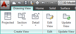
To change the settings on your views, select one. This will activate a contextual Ribbon tab called Drawing View (Figure 24-39), bringing up the tools you need to edit your selected view. Use the Projected command to create new projections from the selected view. The Section command will create a cross-section view. Detail will create a detail view. Edit View allows you to make changes to the hidden lines, scale, and visibility settings.
Figure 24-39 Selecting a view will activate the contextual Drawing View Ribbon tab.
Creating Section Views
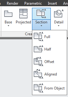
The Section command can create several types of cross sections, but they all work in a similar way. You can create full, half, offset, or aligned sections. You can also create a section based on an object. The Section button in the Ribbon has a flyout that will display these commands, but you can always just click the Section command itself (see Figure 24-40). This will start the Aligned Section command, which should fill most of your needs:
Figure 24-40 Select the Section command or choose a specific type of section to create.
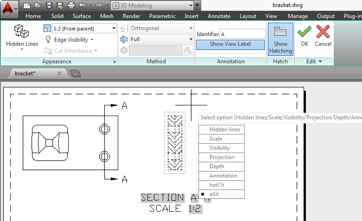
A section has display settings similar to those for the base views but with a few more elements you have to define. Two of the more obvious additional items are the label and the hatching. The Annotation setting controls the label and callouts. The first section of a drawing is typically labeled as A-A. As you insert new sections, AutoCAD will continue down the alphabet automatically for you. The second section created will be labeled B, then C, and so on. Of course, you can change any of these at any time.
As illustrated in Figure 24-41, the section will be labeled. It will be called Section and will display the scale. These items are text fields and can be changed too, or you can turn them off. The label is an Mtext object and can be manipulated just as any other text object. Double-click the label to open the text editor. The hatching in the section is a hatch object and can be edited with the hatch editor. It, too, can be turned off.
Figure 24-41 Section views are edited in the same way as all other view types. They also contain hatch objects and annotation labels.
To change the display features of the section, you can click the Edit View command in the Ribbon and select the section view. (In fact, you can use the Edit View command to make changes to any type of view that you have created.) A contextual Ribbon tab appears. You can change how the section is displayed in the Appearance panel, change the method by which the section is generated in the Method panel, alter the label in the Annotation panel, and toggle the hatch on or off in the Hatch panel.
You can create section styles, similar to dimension styles, by typing viewsectionstyle at the command line. If you have worked with dimension styles, discussed in Chapter 12, “Using Dimensions,” the following process will be second nature:
Creating Detail Views
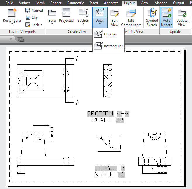
The Detail command, located in the Create View panel in the Layout tab in the Ribbon, creates an enlarged detail view, either circular or rectangular, of a specific area of your model. Follow these steps:
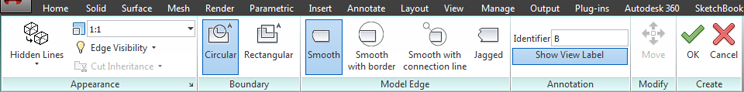
Detail views have settings similar to the settings for the other views, with a few that are unique. Figure 24-42 illustrates the detail view contextual Ribbon tab. The Boundary setting controls whether the detail is a rectangle or circle. The Model Edge setting controls the boundary around the detail; it can be jagged, smooth, smooth with a border, or smooth with a connection line. The remaining settings are the same as for other view types. Views typically inherit the scale from the parent view. Detail views will be “zoomed in” so you can see the details more clearly.
Figure 24-42 While you’re creating a detail view, a contextual Ribbon appears that will provide access to the detail view settings.
Once you have created your views (see Figure 24-43 for a finished set of views), you can always remove them or add more. If the model changes, you can update the views by using the Update View command in the Update panel of the Layout tab. Toggle on the Auto Update setting (also in the Update panel), and whenever the model is changed, the views will automatically update.
Figure 24-43 The Base View command along with the section and detail views can make creating 2D drawings from a 3D model a simple and quick process.
Adding Dimensions and Notes in a Layout
Although we don’t recommend adding dimensions in Paper Space for architectural drawings, doing so may be a good idea for mechanical drawings such as the one in this chapter. By maintaining the dimensions and notes separate from the actual model, you keep these elements from getting in the way of your work on the solid model. You also avoid the confusion of having to scale the text and dimension features properly to ensure that they will plot at the correct size. See Chapter 10, “Adding Text to Drawings,” and Chapter 12 for a more detailed discussion of notes and dimensions.
As long as you set up your Paper Space work area to be equivalent to the final plot size, you can set the dimension and text to the sizes you want at plot time. If you want text ¼″ high, you set your text styles to be ¼″ high.
To include dimensions, make sure you’re in a layout view and then use the dimension commands in the normal way. However, you must make sure full associative dimensioning is turned on. Choose Options from the Application menu to open the Options dialog box, and then click the User Preferences tab. In the Associative Dimensioning group, make sure the Make New Dimensions Associative check box is selected. With associative dimensioning turned on, dimensions in a layout view display the true dimension of the object being dimensioned regardless of the scale setting of the viewport.
If you don’t have the associative dimensioning option turned on and your viewports are set to a scale other than 1 to 1, you have another option: You can set the Annotation Units option in the Dimension Style dialog box to a proper value. The following steps show you how:
You’ve had to complete a lot of steps to get the final drawing, but compared with drawing these views by hand, you undoubtedly saved a great deal of time. In addition, as you’ll see later in this chapter, what you have is more than just a 2D drafted image. With what you created, further refinements are now easy.
Using Visual Styles with a Viewport
In Chapter 21, you saw how you can view your 3D model using visual styles. A visual style can give you a more realistic representation of your 3D model, and it can show off more of the details, especially on rounded surfaces. You can also view and plot a visual style in a layout view. To do so, you make a viewport active and then turn on the visual style you want to use for that viewport. The following exercise gives you a firsthand look at how this is done:
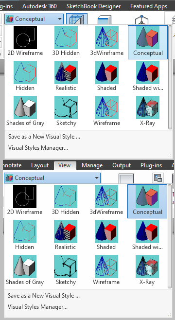
Figure 24-44 The Visual Styles panel and the View panel
You’ve just seen that if you have multiple viewports in a layout, you can change the visual style of one viewport without affecting the other viewports. This can help others visualize your 3D model more clearly.
You’ll also want to know how to control the hard-copy output of a shaded view. For this you use the context menu:
Figure 24-45 The Shade Plot options
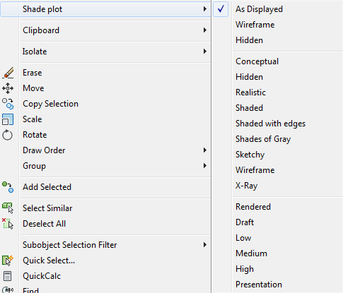
The As Displayed option plots the viewport as it appears in the AutoCAD window. You use this option to plot the currently displayed visual style. Wireframe plots the viewport as a Wireframe view. Hidden plots the viewport as a hidden-line view similar to the view you see when you use the Hide command. Below the Hidden option in the context menu is a list of the available visual styles. At the bottom of the menu is the Rendered option, which plots the view by using the Render feature, described in Chapter 23, “Rendering 3D Drawings.” You can use the Rendered option to plot raytraced renderings of your 3D models.
Remember these options on the context menu as you work on your drawings and when you plot. They can be helpful in communicating your ideas, but they can also get lost in the array of tools that AutoCAD offers.
Visualizing Solids
If you’re designing a complex object, sometimes it helps to be able to see it in ways that you couldn’t in the real world. AutoCAD offers two visualization tools that can help others understand your design ideas.
If you want to show off the internal workings of a part or an assembly, you can use X-Ray Effect, which can be found in the View tab’s Visual Styles panel.
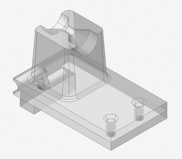
Figure 24-46 shows an isometric view of the bracket using the Realistic visual style and with X-Ray Effect turned on. The color of the bracket has also been changed to a light gray to help visibility. You can see the internal elements as if the object were semitransparent. X-Ray Effect works with any visual style, although it works best with a style that shows some of the surface features (such as the Conceptual or Realistic visual style).
Figure 24-46 The bracket displayed using a Realistic visual style and X-Ray Effect
Another tool to help you visualize the internal workings of a design is the Section Plane command. This command creates a plane that defines the location of a cross section. A section plane can also do more than just show a cross section. Try the following exercise to see how it works:
Figure 24-47 Adding the section plane to your bracket
Select face or any point to locate
section line or [Draw section/Orthographic]:You can move the section plane object along the solid to get a real-time view of the section it traverses. To do this, you need to turn on the Live Section feature. To check whether Live Section is turned on, do the following:
Figure 24-48 Moving the surface plane across the bracket
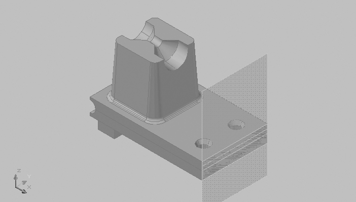
Now you see only a portion of the bracket behind the section plane plus the cross section of the plane, as shown in Figure 24-49. You can have the section plane display the front portion as a ghosted image by doing the following:
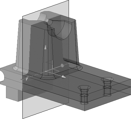
Figure 24-49 The surface plane fixed at a location
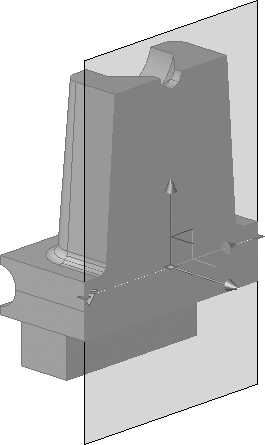
Figure 24-50 The front portion of the bracket is displayed with the Show Cut-Away Geometry option turned on.
You can double-click on the section plane to toggle between a solid view and a cut-away view of the geometry. This toggles the Active Live Sectioning option.
You can also add a jog in the section plane to create a more complex section cut. Here’s how it’s done:
Figure 24-51 Moving the jog in the section plane
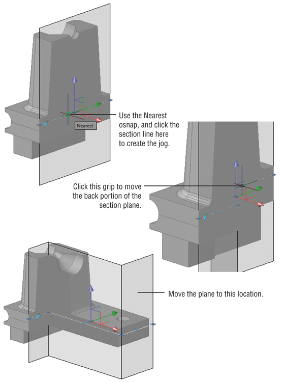
As you can see from this example, you can adjust the section using the grips on the section plane line. You can use the Nearest osnap to select a point anywhere along the section line to a jog. Click and drag the endpoint grips to rotate the section plane to an angle.
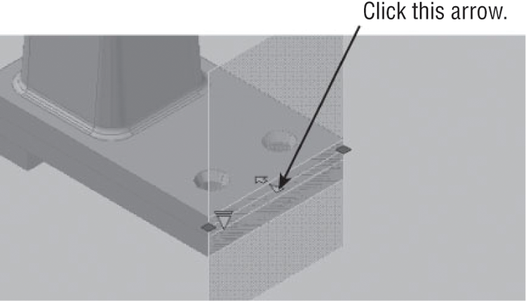
You may have also noticed another arrow in the section plane (see Figure 24-52).
Figure 24-52 The arrow presents additional options for the section plane.
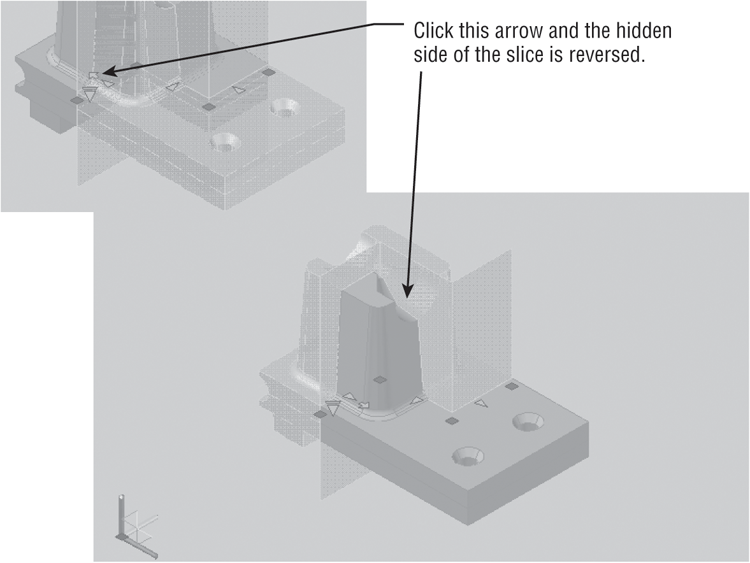
When you click the down-pointing arrow, you see three options for visualizing the section boundary: Section Plane, Section Boundary, and Section Volume.
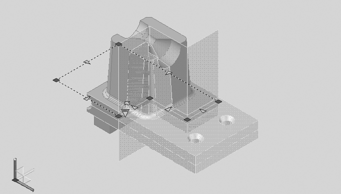
By using these other settings, you can start to include sections through the sides, back, top, or bottom of the solid. For example, if you click the Section Boundary option, another boundary line appears with grips (see Figure 24-53). To see it clearly, you may have to press Esc and then select the section plane again. You can then manipulate these grips to show section cuts along those boundaries.
Figure 24-53 Another boundary line appears with grips when you click the Section Boundary option.
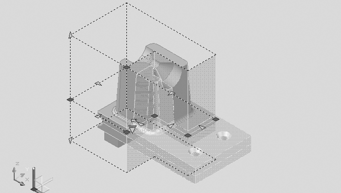
The Section Volume option displays the boundary of a volume along with grips at the top and bottom of the volume (see Figure 24-54). These grips allow you to create a cut plane from the top or bottom of the solid.
Figure 24-54 The boundaries shown using the Section Volume option
Finally, you can get a copy of the solid that is behind or in front of the section plane. Right-click the section plane and choose Generate 2D/3D Section to open the Generate Section/Elevation dialog box. Click the Show Details button to expand the dialog box and display more options (see Figure 24-55).
Figure 24-55 The Generate Section/Elevation dialog box
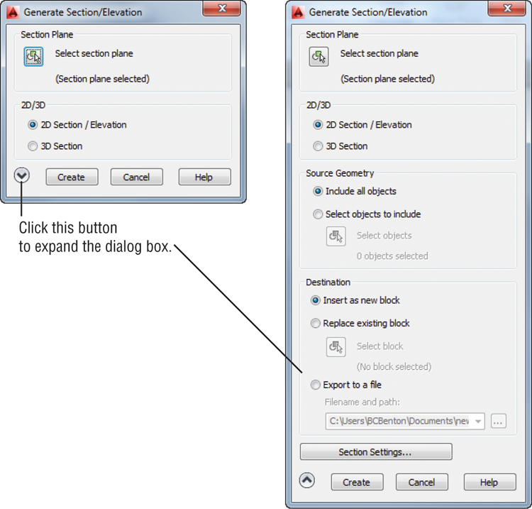
If you select 2D Section/Elevation, a 2D image of the section plane is inserted in the drawing in a manner similar to the insertion of a block. You’re asked for an insertion point, an X and Y scale, and a rotation angle.
The 3D Section option creates a copy of the portion of the solid that is bounded by the section plane or planes, as shown in Figure 24-56.
Figure 24-56 A copy of the solid minus the section area is created using the 3D Section option of the Generate Section/Elevation dialog box.

You can access more detailed settings for the 2D Section/Elevation, 3D Section, and Live Section Settings options by clicking the Section Settings button at the bottom of the Generate Section/Elevation dialog box. This button opens the Section Settings dialog box (see Figure 24-57), which lists the settings for the section feature.
If you create a set of orthogonal views in a layout, the work you do to find a section is also reflected in the layout views (see Figure 24-58).
Figure 24-57 The Section Settings dialog box
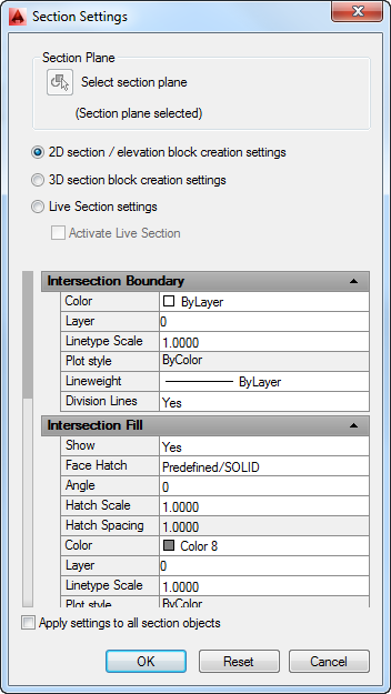
Figure 24-58 A set of orthogonal views in a layout