
Chapter 17
Making “Smart” Drawings with Parametric Tools
Don’t let the term parametric drawing scare you. Parametric is a word from mathematics, and in the context of AutoCAD® drawings, it means that you can define relationships between different objects in a drawing. For example, you can set up a pair of individual lines to stay parallel or set up two concentric circles to maintain an exact distance between the circles no matter how they may be edited.
Parametric drawing is also called constraint-based modeling, and you’ll see the word constraint used in the AutoCAD Ribbon to describe sets of tools. The term constraint is a bit more descriptive of the tools you’ll use to create parametric drawings because when you use them, you are applying a constraint upon the objects in your drawing.
In this chapter, you’ll see firsthand how the parametric drawing tools work and how you might apply them to your needs.
In this chapter, you will learn to:
- Use parametric drawing tools
- Connect objects with geometric constraints
- Control sizes with dimensional constraints
- Use formulas to control dimensions
- Put constraints to use
Why Use Parametric Drawing Tools?
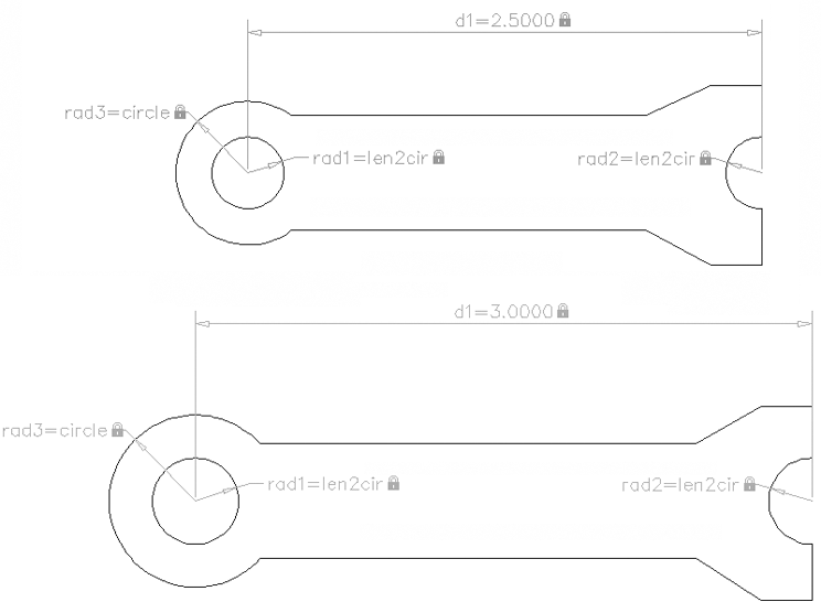
If you’re not familiar with parametric drawing, you may be wondering what purpose it serves. With careful application of the parametric tools, you can create a drawing that you can quickly modify with just a change of a dimension or two instead of actually editing the lines that make up the drawing. Figure 17-1 shows a drawing that was set up so that the arcs and circles increase in size to an exact proportion when the overall length dimension is increased. This approach can save a lot of time if you’re designing several parts that are similar with only a few dimensional changes.
Figure 17-1 The d1 dimension in the top image was edited to change the drawing to look like the one in the lower half.
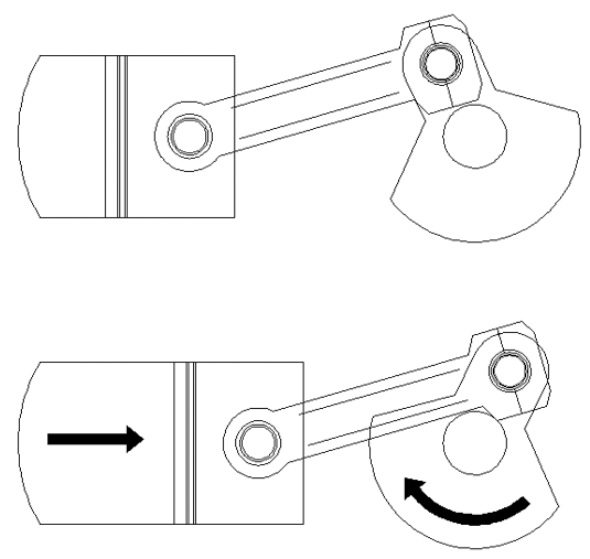
You can also mimic the behavior of a mechanical assembly to test your ideas. The parametric drawing tools let you create linkages between objects so that if one moves, the others maintain their connection like a link in a chain. For example, you can create 3D AutoCAD models of a crankshaft and piston assembly of a car motor (see Figure 17-2) or the parallel arms of a Luxo lamp. If you move one part of the model, the other parts move in a way consistent with a real motor or lamp.
Figure 17-2 Move one part of the drawing and the other parts follow.
Connecting Objects with Geometric Constraints
You’ll start your exploration of parametric drawing by adding geometric constraints to an existing drawing and testing the behavior of the drawing with the constraints in place. Geometric constraints let you assign constrained behaviors to objects to limit their range of motion. Limiting motion to improve editing efficiency may seem counterintuitive, but once you’ve seen these tools in action, you’ll see their benefits.
Using AutoConstrain to Add Constraints Automatically
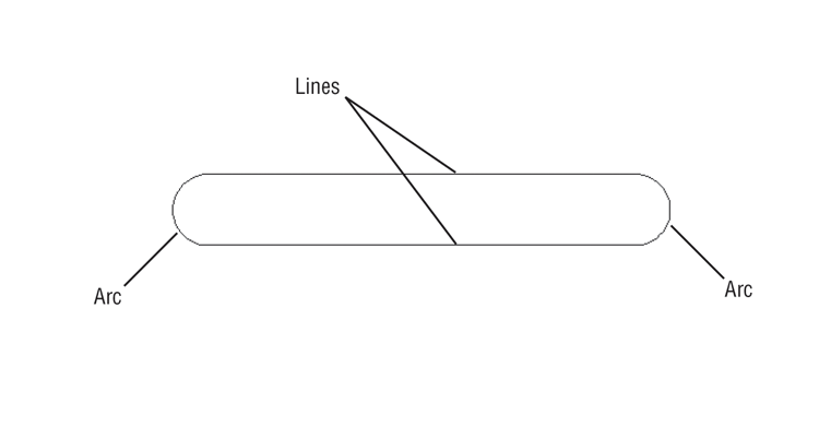
Start by opening a sample drawing and adding a few geometric constraints. The sample drawing is composed of two parallel lines connected by two arcs, as shown in Figure 17-3. These are just lines and arcs and are not polylines.
Figure 17-3 The Parametric01.dwg file containing simple lines and arcs
Here are the steps:

You’ve just used the AutoConstrain command to add geometric constraints to all of the objects in the drawing. You can see a set of icons that indicate the constraints that have been applied to the objects (see Figure 17-4). The AutoConstrain command makes a “best guess” at applying constraints.
Figure 17-4 The drawing with geometric constraints added
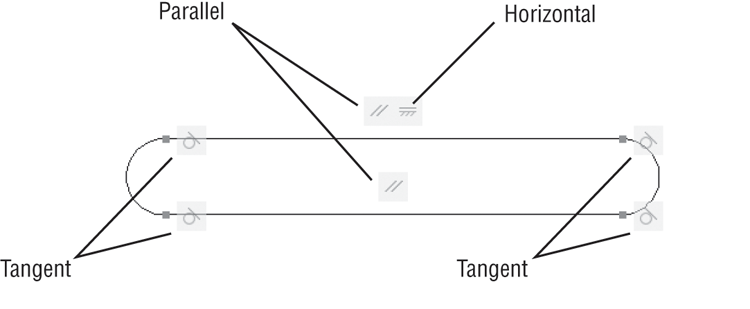
Notice that the constraint icons in the drawing match those you see in the Geometric panel. If you hover your mouse pointer over an icon, you’ll see a tool tip that shows the name of the constraint.
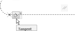
The Tangent constraints that you see at the ends of the lines keep the arcs and the lines tangent to each other whenever the arcs are edited. The Parallel constraint keeps the two lines parallel, and the Horizontal constraint keeps the lines horizontal.
There is one constraint that doesn’t show an icon, but you see a clue to its existence by the small blue squares where the arcs join the lines:
The Coincident constraint makes sure that the endpoints of the lines and arcs stay connected, as you’ll see in the next few exercises.
Editing a Drawing Containing Constraints
Now try editing the drawing to see how these constraints work:
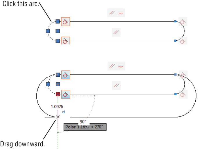
In this exercise, you saw how the Tangent, Parallel, Horizontal, and Coincident constraints worked to keep the objects together while you changed the size of one object. Next, you’ll see what happens if you remove a constraint.
Figure 17-5 Moving the endpoint of one arc causes the other parts of the drawing to follow because of their geometric constraints.
Removing a Constraint
The AutoConstrain tool applied quite a few geometric constraints to the drawing. Suppose you want to remove a constraint to allow for more flexibility in the drawing. In the next exercise, you’ll remove the Parallel constraint and then try editing the drawing to see the results:
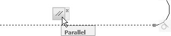
Figure 17-6 Editing the arc with the Parallel constraint removed
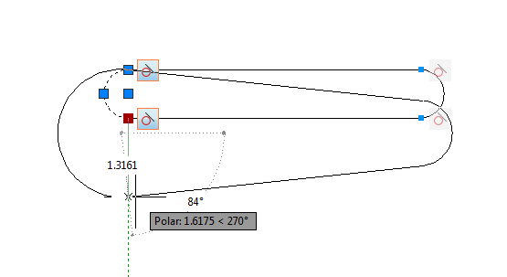
Notice that the top line remains horizontal as you edit the arc. The top line still has the Horizontal constraint. Next try removing the Horizontal constraint:

Figure 17-7 Without the Horizontal constraint, both lines change as the arc is edited.
Notice that lines and arcs remain connected and tangent to each other. This is because the Coincident and Tangent constraints are still in effect.
Adding a Constraint
You’ve seen how the AutoConstrain tool applies a set of constraints to a set of objects. You can also add constraints “manually” to fine-tune the way objects behave. In the next exercise, you’ll add a circle to the drawing and then add a few specific constraints that you’ll select from the Geometric panel:
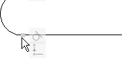
Figure 17-8 Place the circle roughly in the location shown here.
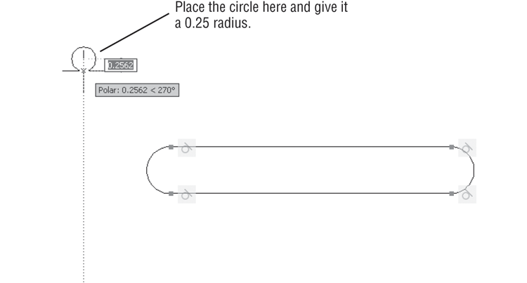
Figure 17-9 The circle is concentric to the arc on the left side.
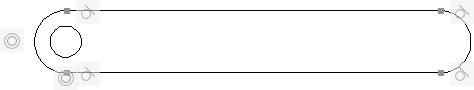
In this exercise, you used the geometric constraint as an editing tool to move an object into an exact location. The Concentric constraint will also keep the circle inside the arc no matter where the arc moves.
Using Other Geometric Constraints
You’ve seen how several of the geometric constraints work. For the most part, each constraint is fairly easy to understand. The Tangent constraint keeps objects tangent to each other. The Coincident constraint keeps the location of objects together, such as endpoints or midpoints of lines and arcs. The Parallel constraint keeps objects parallel.
You have many more geometric constraints at your disposal. Table 17-1 gives you a concise listing of the constraints and their purposes. Note that, with the exception of Fix and Symmetric, all of the constraints affect pairs of objects.
Table 17-1: The geometric constraints
| Name | Use |
| Coincident | Keeps point locations of two objects together, such as the endpoints or midpoints of lines. Allowable points vary between objects, and they are indicated by a red circle marked with an X while points are being selected. |
| Collinear | Keeps lines collinear. The lines need not be connected. |
| Concentric | Keeps circles and arcs concentric. |
| Fix | Fixes a point on an object to a location in the drawing. |
| Parallel | Keeps lines parallel. |
| Perpendicular | Keeps lines or polyline segments perpendicular. |
| Horizontal | Keeps lines horizontal. |
| Vertical | Keeps lines vertical. |
| Tangent | Keeps curves, or a line and curve, tangent to each other. |
| Smooth | Maintains a smooth transition between splines and other objects. The first object selected must be a spline. You can think of this constraint as a tangent constraint for splines. |
| Symmetric | Maintains symmetry between two curves about an axis that is determined by a line. Before using this constraint, draw a line that you will use for the axis of symmetry. You can also use the Fix, Horizontal, or Vertical constraint to fix the axis to a location or orientation. |
| Equal | Keeps the length of lines or polylines equal, or the radius of arcs and circles equal. |
The behavior of the geometric constraints might sound simple, but you may find that they can behave in unexpected ways. With the limited space of this book, we can’t give exercise examples for every geometric constraint, so we encourage you to experiment with them on your own. And have some fun with them!
Using Constraints in the Drawing Process
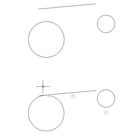
Earlier you saw how the Concentric constraint allowed you to move a circle into a concentric location to an arc. You can use other geometric constraints in a similar way. For example, you can move a line into a collinear position with another line using the Collinear constraint. Or you can move a line into an orientation that’s tangent to a pair of arcs or circles, as shown in Figure 17-10. The top image shows the separate line and circles, and the bottom image shows the objects after applying the Tangent constraint. Note that although the line is tangent to the two circles, its length and orientation does not change.
Figure 17-10 You can connect two circles so that they are tangent to a line by using the Tangent constraint.
Controlling Sizes with Dimensional Constraints
At the heart of the AutoCAD parametric tools are the dimensional constraints. These constraints allow you to set and adjust the dimension of an assembly of parts, thereby giving you an easy way to adjust the size and even the shape of a set of objects.
For example, suppose you have a set of parts that you are drafting, each of which is just slightly different in one dimension or another. You can add geometric constraints and then add dimensional constraints, which will let you easily modify your part just by changing the value of a dimension. To see how this works, try the following exercises.
Adding a Dimensional Constraint
In this first dimensional constraint exercise, you’ll add a horizontal dimension to the drawing you’ve been working on already. The drawing already has some geometric constraints with which you are familiar, so you can see how the dimensional constraints interact with the geometric constraints.
Start by adding a dimensional constraint between the two arcs:

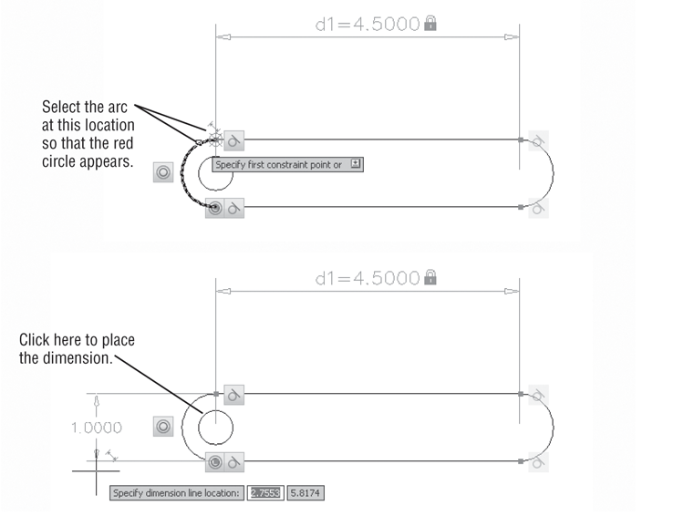
Figure 17-11 Use the Center osnap to select the center of the arc.
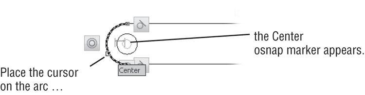
Figure 17-12 Adding the dimensional constraint
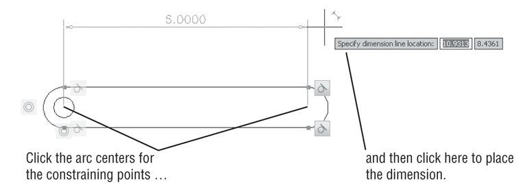
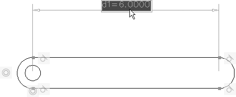
The dimensional constraint appears above the drawing and shows a value of d1=6.0000. The d1 is the name for that particular dimensional constraint. Each dimensional constraint is assigned a unique name, which is useful later when you want to make changes.
Now let’s see how you can use the dimensional constraint you just added.
Editing a Dimensional Constraint
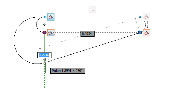
A dimensional constraint is linked to objects in your drawing so that when you modify a dimension value, the objects to which the constraint is linked change. To see how this works, tryediting the part by changing the dimension:
Figure 17-13 Double-click the dimension value.
Next, add a dimension to the arc on the right side:

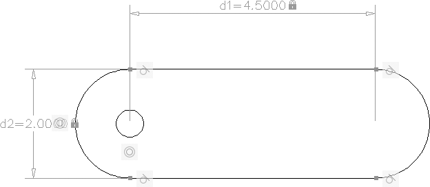
Figure 17-14 Adding a dimensional constraint to the arc
Notice that the new dimensional constraint has been given the name d2. Now try changing the size of the arc using the dimensional constraint:
Figure 17-15 Adjusting the arc dimension
As you can see from this example, you can control the dimensions of your drawing by changing the dimensional constraint’s value. This is a much faster way of making accurate changes to your drawing. Imagine what you would have to do to make these same changes if you didn’t have the geometric and dimensional constraints available.
Using Formulas to Control and Link Dimensions
In the previous exercise, you saw how the dimensional constraint attached to the arc affected the drawing. But in that example, the circle on the left end of the drawing remained unaffected by the change in the arc size. Now suppose that you want that circle to adjust its size in relation to the size of the arc. To do this, you can employ the Parameters Manager and include a formula that manages the size of the circle.
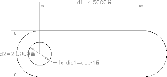
In the following exercise, you’ll add a dimensional constraint to the circle and then apply a formula to that constraint so that the circle will always be one half the diameter of the arc, no matter how the arc is modified.
Start by adding a Diameter constraint to the circle:
Figure 17-16 Adding a Diameter constraint to the circle
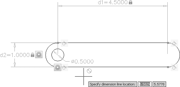
The Diameter constraint you just added is given the name dia1. It controls only the diameter of the circle; you could change the value of that constraint, but it would affect only the circle.
Adding a Formula Parameter
Now let’s add a formula that will “connect” the value of the circle diameter to the diameter of the arc:

Figure 17-17 The Parameters Manager
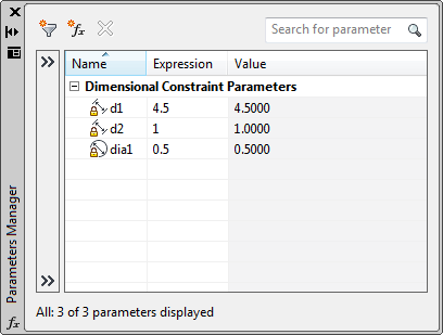
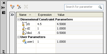
Figure 17-18 Adding an expression to the user1 parameter
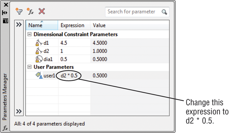
Figure 17-19 Applying the user1 parameter to the dia1 parameter
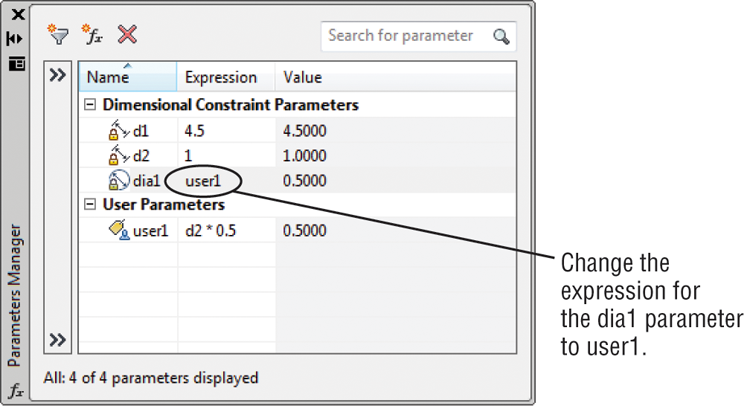
You’ve set up your circle to follow any changes to the width of the part. Now any changes to the d2 dimensional constraint will affect the circle.
Testing the Formula
Try the following to see the parameters in action:
Figure 17-20 Change the d2 parameter and the part changes in size, including the circle.
The part changes in width and the circle also enlarges to maintain its proportion to the width of the part. Here you see that you can apply a formula to a constraint so that it is “linked” to another constraint’s value. In this case, you set the circle’s diameter to follow the width constraint of the part.
In addition, you can adjust the constraint value from the Parameters Manager. You could also have changed the width of the part as before by double-clicking the dimensional constraint for the arc.
Using Other Formulas
In the previous exercise, you used a simple formula that multiplied a parameter, d2, by a fixed value. You used the asterisk to indicate multiplication. You could have used the minus sign in the formula if, for example, you wanted the circle to be an exact distance from the arc. Instead of d2 * 0.5, you could use d2 – 0.125, which would keep the circle 0.125 from the overall width of the part.
You can also choose from a fairly large list of formulas. If you double-click an expression in the Parameters Manager and then right-click, you can select Expressions from the context menu that appears. You can then select from a list of expressions for your parameter (see Figure 17-21).
Figure 17-21 The expressions offered from the Parameters Manager
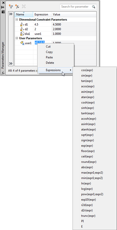
As you can see from the list, you have quite a few expressions from which to choose. We won’t try to describe each expression, but you should recognize most of them from your high school math class.
Editing the Constraint Options
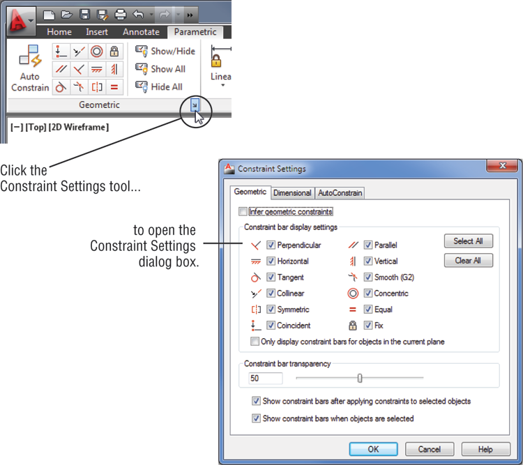
AutoCAD offers a number of controls that you can apply to the constraints feature. Like most other controls, these are accessible through a settings dialog box that is opened from the Ribbon panel title bar. If you click the Constraint Settings tool on the Geometric panel title bar, the Constraint Settings dialog box opens (see Figure 17-22).
You can see that the Constraint Settings dialog box offers three tabs across the top: Geometric, Dimensional, and AutoConstrain. The settings in the Geometric tab let you control the display of the constraint bars, which are the constraint icons you see in the drawing when you add constraints. You can also control the transparency of the constraint bars using the slider near the bottom of the dialog box.
Figure 17-22 The Constraint Settings dialog box showing the Geometric tab
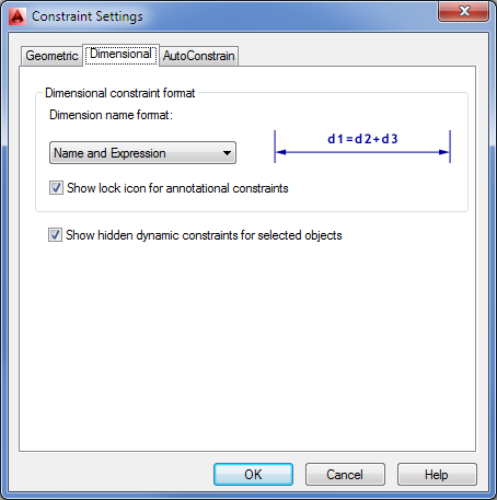
Like the Geometric tab, the Dimensional tab (see Figure 17-23) gives you control over the display of dimensional constraints. You can control the format of the text shown in the dimension and whether dynamic constraints are displayed.
Figure 17-23 The Dimensional tab of the Constraint Settings dialog box
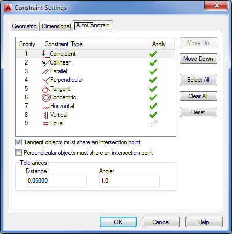
Finally, the AutoConstrain tab (see Figure 17-24) gives you control over the behavior of the AutoConstrain command. You can control the priority of the constraints applied to a set of objects as well as which geometric constraints are allowed.
Figure 17-24 The AutoConstrain tab of the Constraint Settings dialog box
Putting Constraints to Use
So far, you’ve seen some very simple applications of the parametric tools available in AutoCAD. While the parametric tools may seem simple, you can build some fairly elaborate parametric models using the geometric and dimensional constraints you’ve learned about here.
Besides having a drawing of a part that adjusts itself to changes in dimensional constraints, you can create assemblies that will allow you to study linkages and motion. For example, you can create a model of a piston and crankshaft from a gas engine and have the piston and crankshaft move together.
In the next exercise, you’ll look at a drawing that has been established to show just how constraints can be set up to mimic the way a mechanical part behaves:
Figure 17-25 The piston drawing in motion
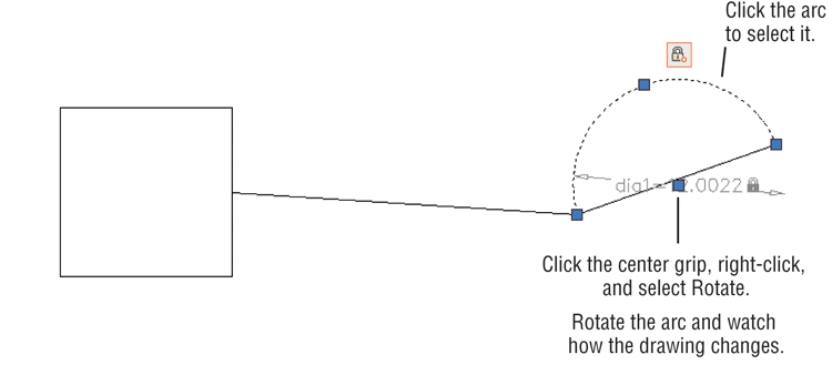
As you can see from this example, you can model a mechanical behavior using constraints. The piston in this drawing is a simple rectangle that has been constrained in both its height and width. A Horizontal constraint has also been applied so that it is capable of moving only in a horizontal direction. The line connecting the piston to the arc is constrained in its length. The Coincident constraint connects it to the piston at one end and the arc at the other end. The arc itself, representing the crankshaft, uses a Diameter constraint, and a Fix constraint is used at its center to keep its center fixed in one location. The net result is that when you rotate the arc, each part moves in unison.