
Chapter 7
Profiles and Profile Views
Profile information is the backbone of vertical design. The Autodesk® AutoCAD® Civil 3D® software takes advantage of sampled data, design data, and external input files to create profiles for a number of uses. Profiles will be an integral part of corridors, as we'll discuss in Chapter 9, “Basic Corridors.” In this chapter we'll look at using profile-creation tools, editing profiles, and generating and editing profile views, and you'll learn ways to get your labels just so.
In this chapter, you will learn to
- Sample a surface profile with offset samples
- Lay out a design profile on the basis of a table of data
- Add and modify individual entities in a design profile
- Apply a standard band set
The Elevation Element
The whole point of a three-dimensional model is to include the elevation element that's been missing for years on two-dimensional plans. But to get there, designers and engineers still depend on a flat 2D representation of the vertical dimension as shown in a profile view (see Figure 7.1).
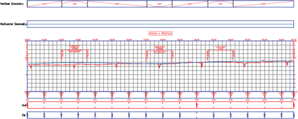
Figure 7.1 A typical profile view of the surface elevation along an alignment
A profile is nothing more than a series of data pairs in a station, elevation format. There are basic curve and tangent components, but these are purely the mathematical basis for the paired data sets. In AutoCAD Civil 3D, you can generate profile information in one of the following five ways:
- Sampling from a Surface Sampling from a surface involves taking vertical information from a surface object every time the sampled alignment crosses a TIN line of the surface. This is perfect for generating a profile for the existing ground.
- Using a Layout to Create a Profile Using a layout to create a profile allows you to input design information, setting critical station and elevation points, calculating curves to connect linear segments, and typically working within design requirements laid out by a reviewing agency.
- Creating a Profile from a File Creating from a file lets you reference a specially formatted text file to pull in the station and elevation pairs. Doing so can be helpful in dealing with other analysis packages or spreadsheet tabular data.
- Creating a Best Fit Profile Similar to the ability to generate a best fit alignment that we discussed in Chapter 6, “Alignments,” you can also create a best fit profile. You may find yourself using this method when you are trying to generate defined geometry for an existing road.
- Creating a Profile from a Corridor You can define a profile by using a corridor's feature line as the source for its definition. This can be helpful for times when you want to display the profiles of the flow line of the curb in the same profile view with the centerline, for example.
The following sections look at the first four methods of creating profiles.
Surface Sampling
![]() Working with surface information is the most elemental method of creating a profile. This information can represent any of the surfaces already in your drawing, such as an existing surface or any number of other surface-derived data sets. Surfaces can also be sampled at offsets, as you'll see in the next series of exercises. Follow these steps:
Working with surface information is the most elemental method of creating a profile. This information can represent any of the surfaces already in your drawing, such as an existing surface or any number of other surface-derived data sets. Surfaces can also be sampled at offsets, as you'll see in the next series of exercises. Follow these steps:
- Open the
0701_ProfileSampling.dwgfile (or the0701_ProfileSampling_METRIC.dwgfile for metric users) shown in Figure 7.2. Remember, all data files can be downloaded from this book's web page at www.sybex.com/go/masteringcivil3d2015.
Figure 7.2 The drawing you'll use for this exercise
 From the Home tab
  Create Design panel, choose Profile Create Surface Profile to display the Create Profile From Surface dialog (Figure 7.3).
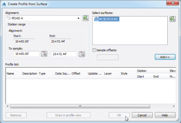
Figure 7.3 The Create Profile From Surface dialog
- Select ROAD A from the Alignment drop-down list if it isn't already selected.
- In the Select Surfaces box, select MC3D2015-EG.
- Click Add to add the centerline profile to the Profile List section.
- Check the box next to Sample Offsets.
- Enter -25, 25 (or -7.62, 7.62 for metric users) to sample at the left and right right-of-way lines and click Add again.
- In the profile list, select the cell in the Style column that corresponds to the negative (left offset) value (see Figure 7.4) to activate the Pick Profile Style dialog. If you need to widen the columns, you can do so by double-clicking the line between the column headings.
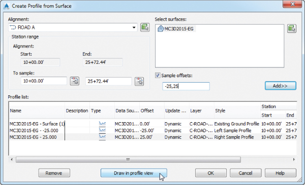
Figure 7.4 The Create Profile From Surface dialog with styles assigned on the basis of the Offset value
- Select the Left Sample Profile option from the drop-down list, and click OK to dismiss the Pick Profile Style dialog.
The style changes from Existing Ground Profile to Left Sample Profile in the table.
- Select the cell in the Style column that corresponds to the positive (right offset) value to activate the Pick Profile Style dialog.
- Select the Right Sample Profile option from the drop-down list, and click OK to dismiss the Pick Profile Style dialog.
- Click Draw In Profile View to dismiss this dialog and open the Create Profile View Wizard, as shown in Figure 7.5.
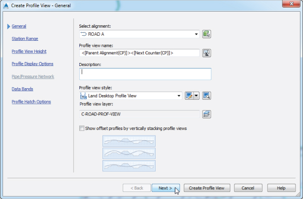
Figure 7.5 The Create Profile View – General : wizard page
- Verify that the Select Alignment drop-down list shows ROAD A and that Land Desktop Profile View is selected in the Profile View Style drop-down list. Click Next.
- On the Create Profile View – Station Range wizard page, verify that the Automatic option has been selected (Figure 7.6). Click Next.

Figure 7.6 The Create Profile View – Station Range wizard page
- On the Create Profile View – Profile View Height wizard page, verify that the Automatic option has been selected (Figure 7.7). Click Next.
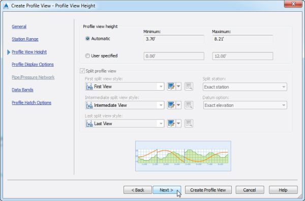
Figure 7.7 The Create Profile View – Profile View Height wizard page
We will examine split profile views in a later exercise.
- On the Create Profile View – Profile Display Options wizard page, look at the settings but do not make any changes (Figure 7.8). Click Next.
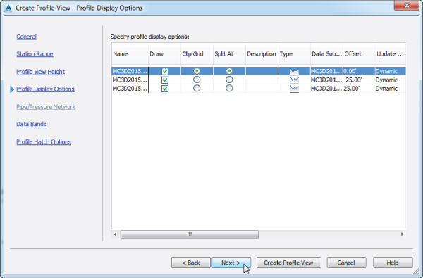
Figure 7.8 The Create Profile View – Profile Display Options wizard page
- On the Create Profile View – Data Bands wizard page, verify that the band set is set to EG-FG Elevations And Stations (Figure 7.9). Notice in the Set Band Properties area that the Profile1 and Profile2 columns are both set to MC3D2015-EG-Surface (1). We will look at data bands in greater detail a bit later.
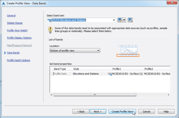
Figure 7.9 The Create Profile View – Data Bands wizard page
Notice that you could continue to click Next to step through the remainder of the wizard; however, you have no need to adjust further options at this time.
- Click the Create Profile View button to dismiss the wizard.
- Pick a point on the screen somewhere to the right of the site to draw the profile view, as shown in Figure 7.10.
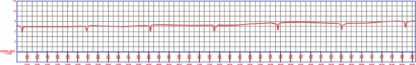
Figure 7.10 The complete profile view for ROAD A
If the Events tab in Panorama appears, telling you that you've sampled data or if an error in the sampling needs to be fixed, then click the green check mark or the X to dismiss Panorama.
Keep the drawing open for the next portion of the exercise.
Profiles are dependent on the alignment they're derived from, so they're stored as profile branches under their parent alignment on the Prospector tab, as shown in Figure 7.11.
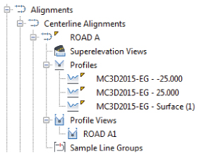
Figure 7.11 Alignment profiles : on the Prospector tab
By maintaining the profiles under the alignments, you make it simpler to review what has been sampled and modified for each alignment. Note that the profiles from surface that you just created are dynamic and continuously update, as you'll see in the next portion of this exercise.
- From the View tab Model Viewports panel, choose the drop-down list on the Viewport Configuration button and select Two: Horizontal.
- Click in the top viewport to activate it.
- On the Prospector tab, expand the Alignments Centerline Alignments branch.
- Right-click ROAD A, and select the Zoom To option.
- Click in the bottom viewport to activate it.
- Expand the Alignments Centerline Alignments ROAD A Profile Views branch.
- Right-click the profile view named ROAD A1, and select Zoom To.
Your screen should now look similar to Figure 7.12.
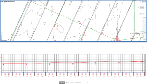
Figure 7.12 Splitting the screen for plan and profile editing
- Click in the top viewport.
- Zoom out so you can see more of the plan view.
- Pick the alignment to activate the grips, and stretch the western end grip to lengthen and/or move the alignment, as shown in Figure 7.13.
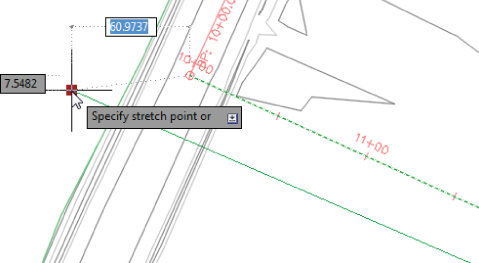
Figure 7.13 Grip-editing the alignment
- Click to complete the edit.
The profile view automatically adjusts to reflect the change in the starting point of the alignment. Note that the offset profiles move dynamically as well.
- Press Ctrl+Z enough times to undo the movement of your alignment and return it to its original location.
- Select the top viewport and then switch back to a single viewport by clicking the viewport controls in the upper-left corner of one of the modelspace viewports and selecting Viewport Configuration List Single.
Save and close the drawing. A finished copy of this drawing is available from the book's website with the filename 0701_ProfileSampling_FINISHED.dwg (0701_ProfileSampling_METRIC_FINISHED.dwg).
By maintaining the relationships between the alignment, the surface, the sampled information, and the offsets, the software creates a much more dynamic feedback system for designers. This system can be useful when you're analyzing a situation with a number of possible solutions, where the surface information will be a deciding factor in the final location of the alignment. Once you've selected a location, you can use this profile view to create a vertical design, as you'll see in the next section.
In the following short exercise you will generate a profile view that displays right to left:
- Open the
0702_ProfileViewMatch.dwgfile (or the0702_ProfileViewMatch_METRIC.dwgfile for metric users), where you will notice that the ROAD A alignment is drawn from right to left while its profile view is shown displayed from left to right. - Select the profile view (grid), and from the Profile View contextual tab Modify View panel, choose Profile View Properties.
- On the Information tab, click the drop-down edit button to the right of the current object style (Land Desktop Profile View) and select Copy Current Selection.
You will learn more about managing and editing these styles in Chapter 19, “Object Styles.”
- On the Information tab, change the Name to Land Desktop Profile View: Right to Left.
You may revise the description if desired.
- In the Profile View Style dialog, on the Graph tab, change the profile view direction to Right To Left.
- Click OK to dismiss the Profile View Style dialog.
- Click OK to dismiss the Profile View Properties dialog.
You may need to move the profile view since the insert point of the profile view will now be in the lower-right corner instead of the lower-left corner as it was previously.
When this exercise is complete, you may close the drawing. A finished copy of this drawing is available from the book's website with the filename 0702_ProfileViewMatch_FINISHED.dwg (0702_ProfileViewMatch_METRIC_FINISHED.dwg).
Changing a profile view style is straightforward, but because of the large number of settings in play with a profile view style, the changes can be dramatic. A profile view style includes information such as labeling on the axis, vertical scale factors, grid clipping, and component coloring.
Using various styles lets you make changes to the view to meet requirements without changing any of the design information associated with the profile. To learn more about editing and creating profile styles, refer to Chapter 19.
Layout Profiles
![]() Working with sampled surface information is dynamic, and the improvement over previous generations of Autodesk civil design software is profound. Moving into the design stage, you'll see how these improvements continue as you look at the nature of creating design profiles. By working with layout profiles as a collection of components that understand their relationships with each other as opposed to independent finite elements, you will realize the power of the AutoCAD Civil 3D software as a design tool in addition to being a drafting tool.
Working with sampled surface information is dynamic, and the improvement over previous generations of Autodesk civil design software is profound. Moving into the design stage, you'll see how these improvements continue as you look at the nature of creating design profiles. By working with layout profiles as a collection of components that understand their relationships with each other as opposed to independent finite elements, you will realize the power of the AutoCAD Civil 3D software as a design tool in addition to being a drafting tool.
You can create layout profiles in two basic ways:
- PVI-Based Layout PVI-based layouts are the most common, using tangents between points of vertical intersection (PVIs) and then applying curve parameters to connect them. PVI-based editing allows editing in a more conventional tabular format.
- Entity-Based Layout Entity-based layouts operate like horizontal alignments in the use of free, floating, and fixed entities. The PVI points are derived from pass-through points and other parameters that are used to create the entities. Entity-based editing allows for the selection of individual entities and editing in an individual component dialog.
You'll work with both methods in the next series of exercises to illustrate a variety of creation and editing techniques. First, you'll focus on the initial layout, and then you'll edit the various layouts.
Layout by PVI
PVI layout is the most common methodology in transportation design. Using long tangents that connect PVIs by derived parabolic curves is a method most engineers are familiar with, and it's the method you'll use in the first exercise:
- Open the
0703_ProfileLayoutPVI.dwg(0703_ProfileLayoutPVI_METRIC.dwg) file.  From the Home tab Create Design panel, choose Profile Profile Creation Tools.
- At the
Select profile view to create profile:prompt, pick the ROAD A profile view by clicking one of the grid lines to display the Create Profile – Draw New dialog. - Set Name to ROAD A FG.
- On the General tab, set Profile Style to Design Profile and Profile Label Set to Complete Label Set, as shown in Figure 7.14.
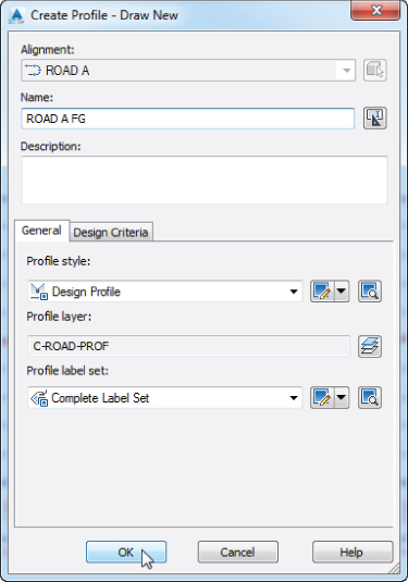
Figure 7.14 The General tab of the Create Profile – Draw New dialog
- Switch to the Design Criteria tab to examine the options provided.
Criteria-based design for profiles is similar to what you learned in Chapter 6 for alignments in that the software compares the design speed to a selected design table (typically AASHTO 2004 in North America) and sets minimum values for curve K values. This can be helpful when you're laying out long highway design projects, but most site and subdivision designers have other criteria to design against. We won't be using design criteria in this exercise, so you can leave everything unchecked.
- Click OK to display the Profile Layout Tools toolbar shown in Figure 7.15.

Figure 7.15 Profile Layout Tools toolbar
Notice that the toolbar is modeless, meaning it stays open even if you do other AutoCAD operations such as Pan or Zoom.
 On the Profile Layout Tools toolbar, click the drop-down arrow next to the Draw Tangents button on the far left.
 Select the Curve Settings option.
The Vertical Curve Settings dialog opens (Figure 7.16).
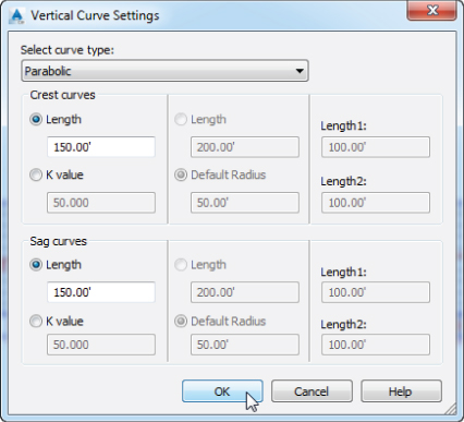
Figure 7.16 The Vertical Curve Settings dialog
The Select Curve Type drop-down menu should be set to Parabolic, and the Length values in both the Crest Curves and Sag Curves areas should be 150.000′ (or 45.720 m for metric users), as shown in Figure 7.16. Selecting a Circular or Asymmetric curve type activates the other options in this dialog.
- Click OK to dismiss the Vertical Curve Settings dialog.
 On the Profile Layout Tools toolbar, click the drop-down arrow next to the Draw Tangents button on the far left again. This time, select the Draw Tangents With Curves option.
- Use a Center Osnap to pick the center of the circle at the far left in the profile view.
- Continue working your way across the profile view, picking the center of each circle left to right with a Center Osnap.
- Right-click or press ↵ after you select the center of the last circle.
- The profile labels will default to a location; however, you can click any of the profile labels and use the grips to move them to a more legible location.
Your drawing should look similar to Figure 7.17.
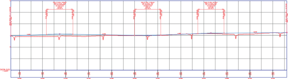
Figure 7.17 A completed layout profile with labels
- Close the Profile Layout Tools toolbar. Save the drawing.
When this exercise is complete, you may close the drawing. A finished copy of this drawing is available from the book's website with the filename 0703_ProfileLayoutPVI_FINISHED.dwg (0703_ProfileLayoutPVI_METRIC_FINISHED.dwg).
The layout profile is labeled with the complete label set you selected in the Create Profile dialog. As you'd expect, this labeling and the layout profile are dynamic. If you select the profile and then zoom in on this profile line, not the labels or the profile view, you'll see something like Figure 7.18.
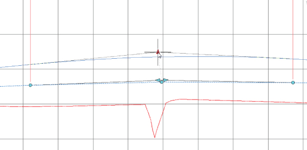
Figure 7.18 The types of grips on a layout profile
The PVI-based layout profiles include the following unique grips:
- Vertical Triangular Grip The vertical triangular grip at the PVI point is the PVI grip. Moving this alters the inbound and outbound tangents, but the curve remains in place with the same design parameters of length and type.
- Angled Triangular Grips The angled triangular grips on either side of the PVI are sliding PVI grips. Selecting and moving moves the PVI, but movement occurs only along the tangent of the selected grip. The curve length isn't affected by moving these grips, but the PVI station and elevation will be, as well as the grade of the other tangent.
- Circular Pass-Through Grips The circular pass-through grips near the PVI and at each end of the curve are curve grips. Moving any of these grips makes the curve longer or shorter without adjusting the inbound or outbound tangents or the PVI point.
Although this simple pick-and-go methodology works for preliminary layout, it lacks a certain amount of control typically required for final design. For that, you'll use another method of creating PVIs:
- Open the
0704_ProfileLayoutPVITransparent.dwg(0704_ProfileLayoutPVITransparent_METRIC.dwg) file. - Verify that the Transparent Commands toolbar (Figure 7.19) is displayed somewhere on your screen. If it is not shown, from the View tab Interface panel, choose Toolbars CIVIL Transparent Commands.

Figure 7.19 The Transparent Commands toolbar
- From the Home tab Create Design panel, choose Profile Profile Creation Tools.
- Pick the ROAD C profile view by clicking one of the grid lines to display the Create Profile – Draw New dialog.
- Set the name to ROAD C FG.
- On the General tab, set Profile Style to Design Profile and Profile Label Set to Complete Label Set. Click OK to display the Profile Layout Tools toolbar.
- On the Profile Layout Tools toolbar, make sure the Curve Settings are set to 150 (45.72 for metric users) by accessing the dialog for these settings, and then click the drop-down arrow next to the Draw Tangents button on the far left and select the Draw Tangents With Curves option, as in the previous exercise.
- Use an End Osnap to snap to the end point of the existing surface profile where this intersects the left edge of the profile view.
 On the Transparent Commands toolbar, select the Profile Station Elevation transparent command.
For those who prefer using the command line, the key-in command for this transparent command is ‘PSE.
- When prompted to select a profile view, click a grid line on the ROAD C profile view to select it.
If you move your cursor within the profile grid area, a vertical red line appears. Notice that the tooltip currently shows the station value of the cursor.
- When prompted for a station, enter 1250 ↵ (or 381 ↵ for metric users) at the command line.
If you move your cursor within the profile grid area, a horizontal line appears (see Figure 7.20), but it can move only vertically along the station just specified.
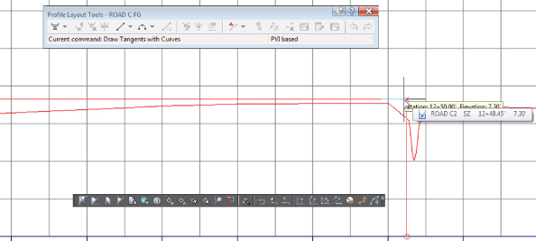
Figure 7.20 Using the Profile Station Elevation transparent command
- When prompted to specify an elevation, enter 8 ↵ (or 2.438 ↵ for metric users) at the command line to set the elevation for the second PVI.
- Press Esc only once.
The Profile Station Elevation transparent command is no longer active, but the Draw Tangents With Curves button that you previously selected on the Profile Layout Tools toolbar continues to be active.
 When prompted to specify a point, select the Profile Grade Station transparent command on the Transparent Commands toolbar.
For those who prefer using the command line, the key-in command for this transparent command is ‘PGS.
Notice that you did not need to select a profile view this time; that's because you are still in the same command (Draw Tangents With Curves in this case). The transparent command will default to the same profile view that was previously selected.
- When prompted to specify the grade, enter -.13 ↵ at the command line for the profile grade.
- When prompted for the station, enter 1520 ↵ (or 463.30 ↵ for metric users) at the command line.
- Press Esc only once to deactivate the Profile Grade Station transparent command.
 When prompted to specify the grade, select the Profile Grade Elevation transparent command on the Transparent Commands toolbar.
For those who prefer using the command line, the key-in command for this transparent command is ‘PGE.
- When prompted to specify the grade, enter 0.31↵ at the command line for the profile grade.
- Enter 8.39 ↵ (or 2.557 ↵ for metric users) for the profile grade elevation.
- Press Esc only once to deactivate the Profile Grade Elevation transparent command.
 When prompted to specify the grade, select the Profile Grade Length transparent command on the Transparent Commands toolbar.
For those who prefer using the command line, the key-in command for this transparent command is ‘PGL.
- When prompted to specify the grade, enter -.19↵ at the command line for the profile grade.
- Enter 200↵ (or 60.96↵ for metric users) for the profile grade length.
- Press Esc only once to deactivate the Profile Grade Elevation transparent command.
- Use an End Osnap to select the end of the existing surface profile on the far-right side of the profile view.
- Press ↵ to complete the profile.
Your profile should look like Figure 7.21.
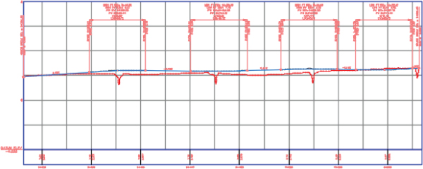
Figure 7.21 A layout profile created using the Transparent Commands toolbar
- Close the Profile Layout Tools toolbar.
When this exercise is complete, you may close the drawing. A finished copy of this drawing is available from the book's website with the filename 0704_ProfileLayoutPVITransparent_FINISHED.dwg (0704_ProfileLayoutPVITransparent_METRIC_FINISHED.dwg).
Using PVIs to define tangents and fitting curves between them is the most common approach to create a layout profile, but you'll look at an entity-based design in the next section.
Layout by Entity
In this exercise you will lay out a design profile using the concepts of fixed, floating, and free entities in much the same way that you used them for laying out alignments in Chapter 6:
- Open the
0705_ProfileEntityLayout.dwg(0705_ProfileEntityLayout_METRIC.dwg) file. - From the Home tab Create Design panel, choose Profile Profile Creation Tools.
- Pick the ROAD B profile view by clicking one of the grid lines to display the Create Profile – Draw New dialog.
- For Name enter ROAD B FG.
- On the General tab, set Profile Style to Design Profile and Profile Label Set to Complete Label Set; then click OK to display the Profile Layout Tools toolbar.
 On the Profile Layout Tools toolbar, click the drop-down arrow next to the Tangent Creation button, and select the Fixed Tangent (Two Points) option.
- Using a Center Osnap, pick the circle at the left edge of the profile view labeled A.
A rubber-band line appears.
- Using a Center Osnap, pick the circle labeled B.
A tangent is drawn between these two circles.
- Using a Center Osnap, pick the circle labeled B again as the start point and the circle labeled C as the endpoint.
A tangent is drawn between these two circles. Notice that the tangent does not automatically continue from the previous two-point fixed tangent; therefore, you have to select the B circle again.
- Using a Center Osnap, pick the circle labeled D as the start point and the circle labeled E as the endpoint.
A tangent is drawn between these two circles.
 On the Profile Layout Tools toolbar, click the drop-down arrow next to the Vertical Curve Creation button and select the More Free Vertical Curves Free Vertical Parabola (PVI Based) option.
Notice that the image shown to the left of the drop-down arrow for the Tangent Creation button and Vertical Curve Creation button will match the last type of entity you selected from the drop-down menu.
- At the
Pick point near PVI or curve to add curve:prompt, pick the circle labeled B as the PVI. - At the
Specify curve length or [Passthrough K]:prompt, enter 150 ↵ (or 45.72 ↵ for metric users) as the curve length. - Press ↵ to end the command.
Your drawing should now look similar to Figure 7.22. Notice that although you have added the tangent between D and E, it is not yet labeled since it is not connected with the main portion of the profile created up until this point.
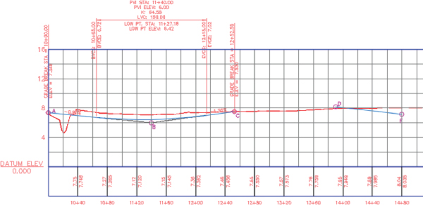
Figure 7.22 Some tangent and vertical curve entities placed on ROAD B
 On the Profile Layout Tools toolbar, click the drop-down arrow next to the Vertical Curve Creation button and select the Free Vertical Curve (Parabola) option.
- When prompted to select the first entity, click the tangent between B and C. Then click the tangent between D and E as the next entity.
Remember to pick the tangent line and not an end circle.
- At the
Specify curve length or [Radius K]:prompt, enter 100 ↵ (or 30.48 ↵ for metric users) as the curve length and press ↵ again to end the command.Notice that with this command the tangents do not have to meet at a PVI, unlike the previous Free Vertical Curve (PVI Based) curve.
 On the Profile Layout Tools toolbar, click the drop-down arrow next to the Vertical Curve Creation button and select the Floating Vertical Curve (Parameter, Through Point) option.
- At the
Select entity to attach to:prompt, select the tangent between D and E to attach the floating vertical curve.Remember to pick the tangent line and not the end circle. Also, you have to select the tangent between the midpoint and the endpoint of the tangent at the circle labeled E. Selecting too close to the endpoint at the circle labeled D will give a result of
End of selected entity already has an attachment. - At the
Enter K value or [Radius]:prompt, enter 73.10 (22.30 for metric users) for the K value and ↵, and then at theSpecify End Point:prompt using the Center Osnap, select the circle labeled F as the end point for the curve.You will notice when using this tool that once you select the first entity and define the parameter, a rubber-band curve appears. If you move the cursor on the wrong side of the tangent endpoint, it will become a large red circle with an X across it indicating that you cannot select that point.
 On the Profile Layout Tools toolbar, click the drop-down arrow next to the Tangent Creation button and select the Float Tangent (Through Point) option.
- At the
Select entity to attach to:prompt, select the curve from E and F making sure to select it between the midpoint of the curve and the circle labeled F to attach the floating tangent.A rubber-band line appears.
- At the
Select through point:prompt, using a Center Osnap, select the circle labeled G. - Press ↵ or right-click to end the Fixed Tangent (Through Point) command; then close the Profile Layout Tools toolbar.
Your drawing should look like Figure 7.23.
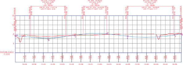
Figure 7.23 Completed profile built using entities
When this exercise is complete, you may close the drawing. A finished copy of this drawing is available from the book's website with the filename 0705_ProfileEntityLayout_FINISHED.dwg (0705_ProfileEntityLayout_METRIC_FINISHED.dwg).
With the entity-creation method, grip editing works in a similar way to other layout methods based on the fixed, floating, and free constraints.
Profile Layout Tools
![]() Although we have touched on many of the available tools in the Profile Layout Tools toolbar, shown in Figure 7.24, there are still many that we have not discussed.
Although we have touched on many of the available tools in the Profile Layout Tools toolbar, shown in Figure 7.24, there are still many that we have not discussed.
- Chained Tangents Creation Tools The Chained Tangents Creation Tools drop-down button contains four options:
- Draw Tangents lays out a profile point to point with no curves.
- Draw Tangent With Curves lays out a profile from point to point with the curve type and length determined from the Curve Settings options.
- Curve Settings sets the type of curve (parabolic, circular, asymmetric) along with specific geometric properties that define each type of curve.
- Convert Free Curve (Through Point) is a new feature introduced with this release that allows free curves that are constrained by using pass-through points to be converted to free curves based on a parameter.
- Insert PVI The Insert PVI button adds a new PVI at the specified location, consequently breaking an existing tangent and generating two new tangents connected to the new PVI.
- Delete PVI The Delete PVI button removes an existing PVI at the specified location, consequently taking two tangents and replacing them with a single tangent.
- Move PVI The Move PVI button allows you to select an existing PVI and relocate it to a specified location while keeping the two existing tangents. You can get the same result by grip-editing the PVI with the vertical triangular grip, as described earlier. In fact, one might argue that the grip-editing approach is better because it shows you a preview of your edit as you make it. The Move PVI command does not.
- Individual Tangents Creation Tools The Individual Tangents Creation Tools Drop-down button contains six tools:
- Fixed Tangent (Two Points)
- Fixed Tangent – Best Fit
- Float Tangent (Through Point)
- Float Tangent – Best Fit
- Free Tangent
- Solve Tangent Intersection
The fixed, float, and free tools are consistent with those discussed in Chapter 6 when we were generating alignments, and therefore many of these options should be self-explanatory. The Solve Tangent Intersection option extends two tangents that do not currently connect to form a PVI.
- Vertical Curves Creation Tools Drop-Down The Vertical Curves Creation drop-down button contains 15 options:
- Fixed Vertical Curve (Three Points)
- Fixed Vertical Curve (Two Points, Parameter)
- Fixed Vertical Curve (Entity End, Through Point)
- Fixed Vertical Curve (Two Points, Grade At Start Point)
- Fixed Vertical Curve (Two Points, Grade At End Point)
- Fixed Vertical Curve – Best Fit
- Floating Vertical Curve (Parameter, Through Point)
- Floating Vertical Curve (Through Point, Grade)
- Floating Vertical Curve – Best Fit
- Free Vertical Curve (Parabola)
- Free Vertical Curve (Circular)—a feature introduced with this release
- Free Vertical Parabola (PVI Based)
- Free Asymmetrical Parabola (PVI Based)
- Free Circular Curve (PVI Based)
- Free Vertical Curve – Best Fit
Once again the fixed, floating, and free terminology should be familiar from Chapter 6. By trying these various options, you will become comfortable with their capabilities and you will find the ones that best fit your design needs.
- Convert AutoCAD Line And Spline The Convert AutoCAD Line And Spline button takes a singular line/spline and converts it into a profile object, either a tangent or a three-point vertical curve, as applicable.
- Tabular PVI Insertion The Tabular PVI insertion button allows you to enter PVI station and elevation information in a table-like dialog, which is helpful if you want to create multiple PVIs at once using station and elevation information. This table allows you to insert PVIs and curves anywhere geometrically possible in the profile. You are not required to enter the PVIs in any specific order when using this method of entry.
- Raise/Lower PVIs The Raise/Lower PVIs button allows you to raise or lower the entire profile or a subset of PVIs within a specified station range. This button will be discussed in a later exercise in the section “Other Profile Edits.”
- Copy Profile The Copy Profile button allows you to copy either the entire profile or a portion of the profile within a specified station range. This button will be discussed later in the section “Other Profile Edits.”
- PVI or Entity Based Selection The PVI or Entity Based selection button allows you to choose to select and display profile layout parameters based on either PVI or entity. By switching the selection to Entity and selecting a curve entity in the Profile Layout Parameters discussed shortly, you will be able to change the parameter constraint. This represents a new enhancement introduced in 2015.
- Select PVI or Entity The Select PVI or Entity button opens the Profile Layout Parameters dialog for the selected PVI or entity.
- Delete Entity The Delete Entity button removes a selected curve or tangent.
- Edit Best Fit Data For All Entities The Edit Best Fit Data For All Entities button turns on the display of a table of the regression data for a profile that was created by best fit. A discussion of best fit profiles is provided in the next section.
- Profile Layout Parameters The Profile Layout Parameters button opens the Profile Layout Parameters dialog, which shows numeric data for editing the selected entity or PVI.
- Profile Grid View The Profile Grid View button opens the Profile Entities tab in Panorama, showing information about all the entities and PVIs in the profile. This is where you have access to make edits on all the entities of the profile.
- Undo/Redo The Undo button reverses that last command and the Redo button reverses the last undo operation. This includes commands and operations that are not part of creating or editing a profile.
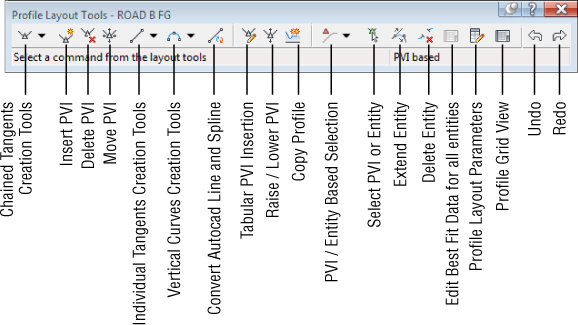
Figure 7.24 Profile Layout Tools toolbar
The Best Fit Profile
You've surveyed along a centerline, and you need to closely approximate the tangents and vertical curves as they were originally designed and constructed.
The Create Best Fit Profile option is found in the Home tab ![]() Create Design panel, on the Profile drop-down. Once you select a profile view, the Create Best Fit Profile dialog appears (Figure 7.25).
Create Design panel, on the Profile drop-down. Once you select a profile view, the Create Best Fit Profile dialog appears (Figure 7.25).
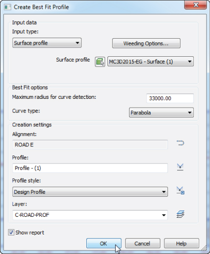
Figure 7.25 Create Best Fit Profile dialog
Similar to the best fit alignment we discussed in Chapter 6, a best fit profile can be based on an Input Type setting of AutoCAD Blocks, AutoCAD 3D Polylines, AutoCAD Points, COGO Points, Surface Profile, or Feature Lines. The most common option is Surface Profile.
The command attempts to run a complex algorithm to determine the best fit profile, including both tangents and vertical curves. However, the only best fit option available for determining vertical curves is the maximum curve radius. The maximum curve radius does not apply in a design that uses parabolic curves, the most common curves found in roadway design. Once the analysis is run, a Best Fit Report is provided; however, unlike the Best Fit command for lines and curves as discussed in Chapter 1, “The Basics,” this command has no options for selecting or deselecting points.
Creating a Profile from a File
Working with profile information in the AutoCAD Civil 3D environment is nice, but it isn't the only place where you can create or manipulate this sort of information. Many programs and analysis packages generate profile information. One common case is the plotting of a hydraulic grade line against a stormwater network profile of the pipes. When information comes from outside the program, it is often output in a variety of formats. If you convert this data to a text file in the format required by AutoCAD Civil 3D, the profile information can be imported directly.
There is a specific format that is required for creating a profile from a text file. Each line is a PVI definition (station and elevation) listed in ascending order. The station should not include the plus character (use 100, not 1+00 or 0+100). Curve information is an optional third bit of data on any line except for the first and last lines in the file. The vertical curve that is created will be a parabolic curve, which is the most popular type of vertical curve. Note that each line is space delimited. Here's one example of a profile text file:
0 550.76
127.5 552.24
200.8 554 100
256.8 557.78 50
310.75 561
In this example, the third and fourth lines include the curve length as the optional third piece of information. The only inconvenience of using this input method is that the information in Civil 3D doesn't directly reference the text file. Once the profile data is imported, no dynamic relationship exists with the text file, but other methods can be used to edit the profile once imported.
In this exercise, you'll import a small text file to see how the function works:
- Open the
0706_ProfilefromFile.dwg(0706_ProfileFromFile_METRIC.dwg) file.  From the Home tab Create Design panel, choose Profile Create Profile From File.The Import Profile From File – Select File dialog appears.
- Browse to and select the
0706_ProfileFromFile.txtfile (or the0706_ProfileFromFile_METRIC.txtfile for metric users), and click Open to display the Create Profile – Draw New dialog. - For Alignment, choose ROAD G, and set Name to ROAD G FG.
- On the General tab, set Profile Style to Design Profile and Profile Label Set to Complete Label Set; then click OK.
Your drawing should look like Figure 7.26. The ROAD G profile view should be updated to reflect the newly imported design profile for the specified alignment.
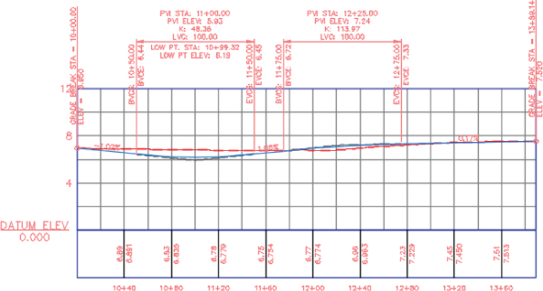
Figure 7.26 Completed profile created from a file
When this exercise is complete, you may close the drawing. A finished copy of this drawing is available from the book's website with the filename 0706_ProfileFromFile_FINISHED.dwg (0706_ProfileFromFile_METRIC_FINISHED.dwg).
Now that you've tried the three main ways of creating profiles, you'll edit a profile.
Editing Profiles
The methods just reviewed let you quickly create profiles. You saw how sampled profiles reflect changes in the surface along the parent alignment and how to lay out a design profile using a few different techniques. You also imported a text file with profile information. In all these cases, you just left the profile as originally designed with no analysis or editing.
In the following sections, you will begin to look at some of the profile-editing methods available. The most basic is a more precise grip-editing methodology, which you'll learn about first. Then you'll see how to modify the PVI-based layout profile, how to change out the components that make up a layout profile, and how to use some other miscellaneous editing functions.
Grip-Editing Profiles
Once a profile layout is in place, sometimes a simple grip edit will suffice. But for precision editing, you can use the grips along with transparent commands or dynamic input, as in this short exercise:
- Open the
0707_ProfileEditing.dwg(0707_ProfileEditing_METRIC.dwg) file. - Zoom to the ROAD D profile view and pick the ROAD D FG profile (the blue line) to activate its grips.
- Locate the PVI around Sta. 19+50 (or 0+594.36 for metric users) and pick the vertical triangular grip on the vertical crest curve to begin a grip stretch of the PVI, as shown in Figure 7.27.
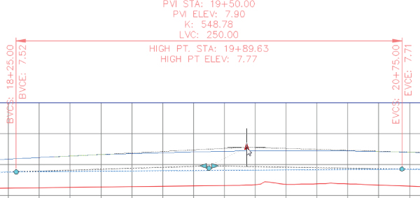
Figure 7.27 Grip-editing a PVI
The command line states
Specify stretch point or [Base point Copy Undo eXit]:.  On the Transparent Commands toolbar, select the Profile Station Elevation command. That's ‘PSE for the command-line users.
- At the
Select a profile view:prompt, pick a grid line on the ROAD D profile view to select. - At the
Specify station:prompt, enter 1975 ↵ (or 601.98 ↵ for metric users). - At the
Specify elevation:prompt, enter 7.50↵ (or 2.286↵ for metric users). - Click the vertical triangular grip for the PVI near station 14+00 (or 0+426.72 for metric users).
 If dynamic input is not turned on already, click the Dynamic Input icon at the bottom of your screen if available, or press the F12 key to enable it.
You should see two editable tooltips on your screen, one for station and one for elevation. You may need to zoom out to see them.
- Enter 1425 ↵ (or 434.34 ↵ for metric users).
When this exercise is complete, you may save the drawing, but keep it open for the following exercise. A copy of this drawing at this stage is available from the book's web page with the filename 0707_ProfileEditingGrips_FINISHED.dwg (0707_ProfileEditingGrips_METRIC_FINISHED.dwg).
The grips can go from quick-and-dirty editing tools to precise editing tools when you use them in conjunction with the transparent commands or dynamic input. They lack the ability to precisely control a curve length, though, so you'll look at editing a curve next.
Editing Profiles Using Profile Layout Parameters
Beyond the simple grip edits, but before changing out the components of a typical profile, you can modify the values that generate an individual component. In this exercise, you'll use the Profile Layout Parameters dialog to modify the curve properties on your design profile:
- Continue working on the previous file, or open the
0707_ProfileEditingGrips_FINISHED.dwg(0707_ProfileEditingGrips_METRIC_FINISHED.dwg) file. - Zoom to the ROAD D profile view and pick the ROAD D FG profile (the blue line) to activate the Profile contextual tab.
- From the Profile contextual tab Modify Profile panel, choose Geometry Editor.
 On the Profile Layout Tools toolbar, click the Profile Layout Parameters button to open the Profile Layout Parameters dialog, and place the dialog somewhere on your screen so that you can still see the profile view.
 On the Profile Layout Tools toolbar, click the Select PVI button.
If the Select Entity button is showing on the toolbar instead, from the PVI /Entity Based selection button select the PVI Based option.
- Zoom in to click near the PVI at station 34+70 (or 1+057.66 for metric users) to populate the Profile Layout Parameters dialog (Figure 7.28).
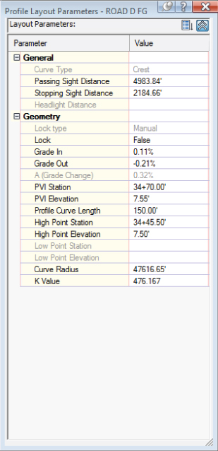
Figure 7.28 The Profile Layout Parameters dialog
Values that can be edited are in black; the rest, shown grayed out, are mathematically derived and can be of some design value but can't be directly modified. The two buttons at the top of the dialog adjust how much information is displayed. The one on the left is the Show More/Show Less button, and the one on the right is the Collapse All Categories/Expand All Categories button.
- In the Profile Layout Parameters dialog, change the K value to 500 ↵ (or 152.4 ↵ for metric users). Notice that the curve changes but the label does not update. This is because you are still in the command. Once you end the command, all appropriate labels will update.
- Change the selection to Entity Based from the PVI/Entity Based Selection drop-down of the toolbar. Click the PVI/Entity Selection button and select the curve at station 38+05 (or 1+159.76 for metric users) to repopulate the Profile Layout Parameters dialog with that curve's data.
- In the Profile Layout Parameters dialog, change Parameter Constraint Lock to False, thus enabling the choice of constraints. In the Constraint Type Desc field, change the value to Through Point. On making this change you will notice that all the other settings are grayed out, leaving you with the option of defining only the Through Point Station and Elevation parameters. Change the station to 38+10 and the elevation to 7.00 (1+161.28 for station and 2.134 for elevation for metric users).
The ability to change the parameter constraint is a new enhancement introduced with this release.
- Close the Profile Layout Parameters dialog by clicking the X in the upper-right corner and press Enter to exit selection mode. Close the Profile Layout Tools toolbar as well.
When this exercise is complete, you may save the drawing, but keep it open for the following exercise. A copy of this drawing at this stage is available from the book's web page with the filename 0707_ProfileEditingParameter_FINISHED.dwg (0707_ProfileEditingParameter_METRIC_FINISHED.dwg).
Editing Profiles Using Profile Grid View
In this exercise, you'll use the Profile Grid View command to view and modify the profile within Panorama:
- Continue using the file from the previous exercise, or if you did not complete the previous exercise, open the
0707_ProfileEditingParameter_FINISHED.dwg(0707_ProfileEditingParameter_METRIC_FINISHED.dwg) file.If you have closed the Profile Layout Tools toolbar, click the ROAD D FG profile, and then from the Profile: ROAD D FG contextual tab
Modify Profile panel, click Geometry Editor.  On the Profile Layout Tools toolbar, change the selection to PVI Based from the PVI/Entity Based Selection drop-down if it is not already set to that mode.
 Click the Profile Grid View tool to activate the Profile Entities tab in Panorama.Panorama allows you to view all the profile components at once, in a compact form.
- Scroll right in Panorama until you see the Profile Curve Length column.You can show and hide columns by right-clicking the column headings. You can also resize the columns by dragging the breaks between the columns or by double-clicking the break between two columns to autosize to the column contents.
- Double-click the Profile Curve Length value for Entity No. 5 (see Figure 7.29) and change the value from 300 to 250 (or from 91.44 to 76.2 for metric users).
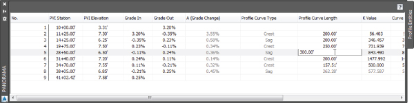
Figure 7.29 Direct editing of the curve length in Panorama
- Close Panorama and the Profile Layout Tools toolbar, and zoom out to review your edits.
Your complete profile should now look like Figure 7.30.
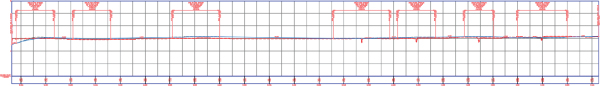
Figure 7.30 The completed editing of the curve length in the layout profile
When this exercise is complete, you may save the drawing, but keep it open for the following exercise. A copy of this drawing at this stage is available from the book's web page with the filename 0707_ProfileEditingGrid_FINISHED.dwg (0707_ProfileEditingGrid_METRIC_FINISHED.dwg).
You can use these tools to modify the PVI points or tangent parameters, but they won't let you add or remove an entire component. You'll do that in the next section.
Component-Level Editing
In addition to editing basic parameters and locations, sometimes you have to add or remove entire components. In this exercise, you'll delete a curve, remove a PVI, insert a new PVI, and add a new curve into the layout profile:
- Continue using the file from the previous exercise, or if you did not complete the previous exercise, open the
0707_ProfileEditingGrid_FINISHED.dwg(0707_ProfileEditingGrid_METRIC_FINISHED.dwg) file.If you have closed the Profile Layout Tools toolbar, click the ROAD D FG profile, and then from the Profile: ROAD D FG contextual tab
Modify Profile panel, click Geometry Editor.  On the Profile Layout Tools toolbar, click the Delete Entity button.
- Pick the curve near the 31+40 station (or the 0+957.07 station for metric users) and right-click or press ↵ to end the command.
The profile is adjusted accordingly. Since the deleted curve was defined as a free curve, on deletion the tangents will be still connected to each other by means of the PVI.
 On the Profile Layout Tools toolbar, click the Delete PVI button. Pick a point near the PVI that resulted from the deletion of the previous curve. Right-click or press ↵ to end the command. The PVI is deleted, and the layout is updated.
 On the Profile Layout Tools toolbar, click the Insert PVI button. At the prompt, using the transparent command for Profile Station and Elevation ('PSE) select the ROAD D profile view and define the new PVI at station 24+00 (0+731.52 for metric users) and the elevation of 5.25 (1.60 for metric users). Press Esc twice, once to exit the transparent command and again to exit the Insert PVI command.
 On the Profile Layout Tools toolbar, expand the Vertical Curves Creation Tools, and from the More Free Vertical Curves section, select Free Asymmetrical Parabola (PVI Based). At the prompt for the PVI click the screen in the vicinity of the previously created PVI at station 24+00 (0+731.52 for metric users). At the
 Specify Length1:prompt, enter 150 (45.72 for metric users) and click Enter. At theSpecify Length2:prompt, enter 100 (30.48 for metric users) and press Enter. Right-click or press the Enter key again to end the command. Close the toolbar.Your layout should update to reflect the new changes, and the drawing should look similar to Figure 7.31.
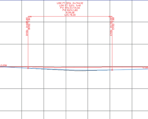
Figure 7.31 The completed editing of the curve using component-level editing
When this exercise is complete, you may save the drawing, but keep it open for the following exercise. A copy of the drawing at this stage is available from the book's web page with the filename 0707_ProfileEditingComponent_FINISHED.dwg (0707_ProfileEditingComponent_METRIC_FINISHED.dwg). Editing profiles using any of these methods gives you precise control over the creation and layout of your vertical design. In addition to these fine-tuning tools, there are other tools worth investigating, and you'll look at them next.
Other Profile Edits
Some handy tools exist on the Profile Layout Tools toolbar for performing specific actions. These tools aren't normally used during the preliminary design stage, but they come into play as you're working to create a final design for grading or corridor design. They include raising or lowering a whole layout in one shot, as well as copying profiles. The 2015 release introduces a new tab within the Profile Properties dialog that allows users to control the locking of the vertical alignment to the horizontal alignment geometry points. You will experiment with all these options in the following exercise:
- Continue using the file from the previous exercise, or if you did not complete the previous exercise, open the
0707_ProfileEditingComponent_FINISHED.dwg(0707_ProfileEditingComponent_METRIC_FINISHED.dwg) file.If you have closed the Profile Layout Tools toolbar, click the ROAD D FG profile, and then from the Profile: ROAD D FG contextual tab
Modify Profile panel, click Geometry Editor.  On the Profile Layout Tools toolbar, click the Copy Profile button to display the Copy Profile Data dialog, shown in Figure 7.32.
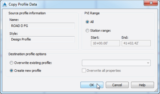
Figure 7.32 The Copy Profile Data dialog
- Click OK to create a new layout profile directly on top of ROAD D FG.
- In Prospector, expand the Alignments Centerline Alignments ROAD D Profiles branch to see that a profile named ROAD D FG [Copy] has been added.
- Press Esc to clear the selection of the original profile, and then click the profile again to select it. This time the ROAD D FG [Copy] profile is selected because it is on top. The Profile Layout Tools toolbar now references the new profile.
 On the Profile Layout Tools toolbar, click the Raise/Lower PVIs button to display the Raise/Lower PVI Elevation dialog, shown in Figure 7.33.
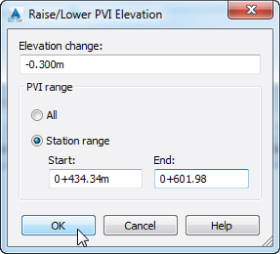
Figure 7.33 The Raise/Lower PVI Elevation dialog
- Set Elevation Change to -1 (or -0.3 for metric users).
- Click the Station Range radio button, and set the Start value to 14+25 (or 0+434.34 for metric users) and the End value to 19+75 (0+601.98 for metric users) to modify the profile in between the starting and ending PVIs.
- Click OK to dismiss the Raise/Lower PVI Elevation dialog.
Generating a copy is useful if you want to remember a conceptual profile layout but would like to experiment with a different layout. The copies do not stay dynamically related to one another.
Let's continue to explore, turning now to the new enhancement to Profile Properties.
- Switch the modelspace to a two-viewport layout from the View tab Model Viewports panel Viewport Configuration drop-down by selecting Two: Horizontal Setup. Make sure that on the top viewport you zoom to the ROAD D alignment, while on the bottom viewport you have the ROAD D profile view.
- Select ROAD D FG either from the profile view or through Prospector and access the Profile Properties dialog. The new Profile Locking tab is shown in Figure 7.34.
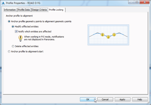
Figure 7.34 The Profile Locking tab of the Profile Properties dialog allows you to lock your vertical alignment to the horizontal geometry points.
Here you have the option of locking the vertical alignment (profile) to the horizontal alignment's geometry points. When locked, upon any changes to the horizontal alignment, the affected profile's entities will be modified either through deletion or a change in their parameters to keep the profile vertical geometry in sync with the horizontal alignment.
- Close the Profile Properties dialog; then in plan view zoom to the curve around station 28+00 (0+853 for metric users). Grip-edit the alignment's curve by selecting the triangular grip, sliding it toward the inside of the curve as shown in Figure 7.35, and clicking a new location not too far from the original location.
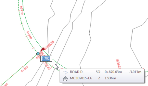
Figure 7.35 Grip-editing the alignment curve by sliding the triangular grip toward the inside of the curve
- Upon editing the alignment, you will notice that in the profile view, for the entities affected by this change, warning signs are displayed, as shown in Figure 7.36. These warning signs let you know that changes have been applied to the entities of the profile in order to maintain the sync of start and end stations with the alignment.
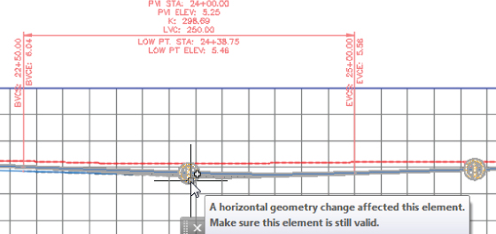
Figure 7.36 On alignment change, warning signs are displayed for the items affected by the change.
If you are used to the profile not being locked with the horizontal alignment, you'll notice changes. Namely, with Profile Locking on, you will notice that even if the alignment changed its length as reflected in the plan and profile views, the design profile ends are tied to the new beginning and end stations for the alignment, and the properties for the entities in between are modified to accommodate this change.
When this exercise is complete, you may save and close the drawing. A finished copy of this drawing at this stage is available from the book's web page with the filename 0707_ProfileEditingOther_FINISHED.dwg (0707_ProfileEditingOther_METRIC_FINISHED.dwg).
Using the layout and editing tools discussed in these sections, you should be able to create profiles for many different types of designs.
Up to now, you have learned how to use some of the available tools for modifying profiles, but you might be wondering about intersecting roads and how their profiles will interact with one another. Have no fear; we are going to discuss those later in Chapter 10, “Advanced Corridors, Intersections, and Roundabouts,” when we discuss corridor intersections.
Profile Views
![]() Working with vertical data is an integral part of building the model. Once profile information has been created in any number of ways, displaying it to make sense is another task. It can't be stated enough that profiles and profile views are not the same thing. The profile view displays the profile data. A single profile can be shown in an infinite number of views, with different grids, exaggeration factors, labels, or linetypes. In the following sections, you'll look at the various methods available for creating profile views.
Working with vertical data is an integral part of building the model. Once profile information has been created in any number of ways, displaying it to make sense is another task. It can't be stated enough that profiles and profile views are not the same thing. The profile view displays the profile data. A single profile can be shown in an infinite number of views, with different grids, exaggeration factors, labels, or linetypes. In the following sections, you'll look at the various methods available for creating profile views.
Creating Profile Views during Sampling
The easiest way to create a profile view is to draw it as an extended part of the surface-sampling procedure, as shown in the first exercise in this chapter. By combining the profile-sampling step with the creation of the profile view, you avoid one more trip to the menus. This is the most common method of creating a profile view, but we'll look at manual creation in the next section.
Creating Profile Views Manually
Once an alignment has profile information associated with it, any number of profile views might be needed to display the proper information in the right format. To create a second, third, or even tenth profile view once the sampling is done, you must use a manual creation method. In this exercise, you'll create a profile view manually for an alignment that already has a surface-sampled profile associated with it:
- Open the
0708_ManualProfileView.dwg(0708_ManualProfileView_METRIC.dwg) file.  From the Home tab Profile & Section Views panel, choose Profile View Create Profile View to display the Create Profile View Wizard.
This is the same wizard that was discussed in the surface-sampling example.
- In the Select Alignment text box, select ROAD G from the drop-down list.
- Set the Profile View name as ROAD G Full Grid.
- In the Profile View Style drop-down list, select the Full Grid style.
- Click the Create Profile View button and pick a point onscreen to draw the profile view, as shown in Figure 7.37.
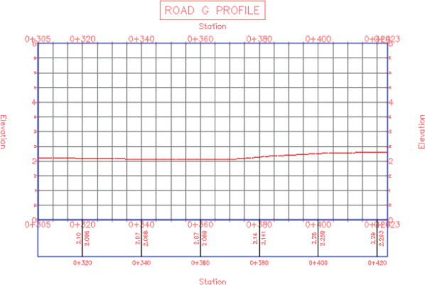
Figure 7.37 The completed profile view of ROAD G using the Full Grid profile view style
When this exercise is complete, you may save the drawing. A copy of this drawing at this stage is available from the book's web page with the filename 0708_ManualProfileView_FINISHED.dwg (0708_ManualProfileView_METRIC_FINISHED.dwg).
Using this creation method, you've made a short, simple profile view, but in the next exercise you will look at a longer alignment as well as some more of the options available in the Create Profile View Wizard.
Splitting Views
Dividing up the data shown in a profile view can be time consuming. The Profile View Wizard is used for simple profile view creation, but the wizard can also be used to create manually limited profile views, staggered (or stepped) profile views, multiple profile views with gaps between the views, and stacked profiles (aka three-line profiles). You'll now look at these variations on profile view creation.
Creating Manually Limited Profile Views
Continuous profile views like the ones you made in the exercises prior to this point work well for design purposes, but they are often unusable for plotting or documentation purposes. In this exercise, you'll use the Profile View Wizard to create a manually limited profile view. This variation will allow you to control how long and how high each profile view will be, thereby making the views easier to plot:
- Open the
ProfileViewsSplit.dwgfile (or theProfileViewsSplit_METRIC.dwgfile). - From the Home tab Profile & Section Views panel, choose Profile View Create Profile View to display the Create Profile View Wizard.
- Verify that the Select Alignment drop-down list shows Frontenac Drive, Profile Name is set to Frontenac Drive Limited Full Grid, and Full Grid is selected in the Profile View Style drop-down list; then click Next.
- On the Station Range wizard page, select the User Specified Range radio button.
- Enter 0 for the start station and 800 for the end station (or 0 and 245 for metric users), as shown in Figure 7.38. It isn't necessary to include the + when entering station data.
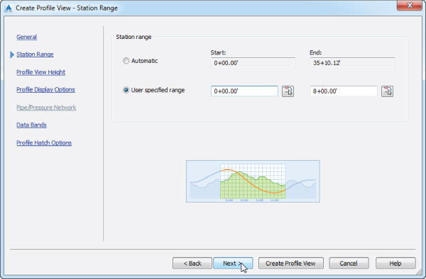
Figure 7.38 The start and end stations for the user-specified : profile view
Notice that the preview picture now shows a clipped portion of the total profile.
- Click Next.
- On the Profile View Height wizard page, select the User Specified radio button.
- Set the minimum height to 1030 and the maximum height to 1060 (or 314 and 322 for metric users). It isn't necessary to include the foot mark (') or m for meters when entering elevations.
- Click the Create Profile View button and pick a point onscreen to draw the profile view.
Your screen should look similar to Figure 7.39.

Figure 7.39 Applying user-specified station and height values to a profile view
When this exercise is complete, you may save the drawing, but keep it open for the following exercise. A copy of the drawing at this stage is available from the book's web page with the filename
0709_ManualLimitedProfileView_FINISHED.dwg(0709_ManualLimitedProfileView_METRIC_FINISHED.dwg).
Creating Staggered Profile Views
When large variations occur in profile height, the profile view must often be split just to keep from wasting much of the page with empty grid lines. In this exercise, you use the Profile View Wizard to create a staggered, or stepped, view:
- Continue using the file from the previous exercise, or if you did not complete the previous exercise, open the
0709_ManualLimitedProfileView_FINISHED.dwg(0709_ManualLimitedProfileView_METRIC_FINISHED.dwg) file. - From the Home tab Profile & Section Views panel, choose Profile View Create Profile View to display the Create Profile View Wizard.
- Verify that the Select Alignment drop-down list shows RM2222, Profile Name is set to RM2222 Staggered Full Grid, and Full Grid is selected in the Profile View Style drop-down list; then click Next.
- Verify that Station Range is set to Automatic to allow the view to show the full length, and click Next.
- In the Profile View Height field, select the User Specified option and set the values to 880 and 970 (or 268 and 294 for metric users), as shown in Figure 7.40.
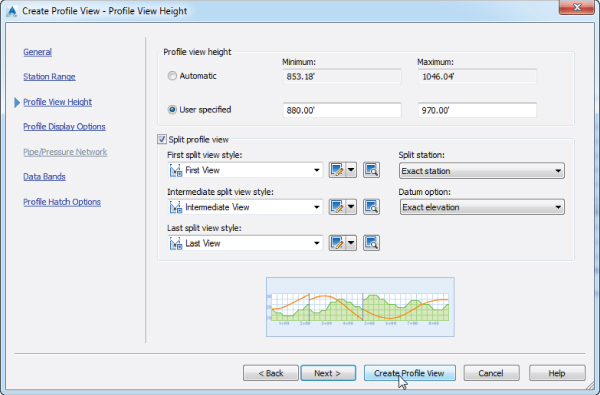
Figure 7.40 Split Profile View settings
- Check the Split Profile View option and set the view styles to First View, Intermediate View, and Last View, as shown in Figure 7.40.
- Click the Create Profile View button and pick a point onscreen to draw the staggered display, as shown in Figure 7.41.
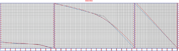
Figure 7.41 A staggered (stepped) split : profile view created via the wizard
The profile view is split into views according to the settings that were selected in the Create Profile View Wizard in step 6. The first portion of the profile view shows the profile from 0 to the station where the elevation change of the profile exceeds the limit for height. If more splits were required, the command would have created them accordingly. Each of these portions is part of the same profile view and can be adjusted via the Profile View Properties dialog. The profile view splits can be controlled manually on the Elevations tab of the Profile View Properties dialog box. Here you can add and remove splits, control the station at which a given split occurs, and control the datum elevation at each split station by changing the Split Profile View option to Manual (see Figure 7.42).
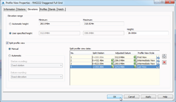
Figure 7.42 The Elevations tab of the Profile View Properties dialog showing manual control of a split profile view
When this exercise is complete, you may save the drawing, but keep it open for the following exercise. A copy of the drawing at this stage is available from the book's web page with the filename 0709_StaggeredProfileView_FINISHED.dwg (0709_StaggeredProfileView_METRIC_FINISHED.dwg).
Creating Gapped Profile Views
Profile views must often be limited in length and height to fit a given sheet size. Gapped views are a way to show the entire length and height of the profile, by breaking the profile into different sections with gaps, or spaces, between each view.
When you are using the Plan Production tools (covered in Chapter 15, “Plan Production”), the gapped profile views are automatically created.
In this exercise, you will use a variation of the Create Profile View Wizard called the Create Multiple Profile Views Wizard to create gapped views automatically:
- Continue using the file from the previous exercise, or if you did not complete the previous exercise, open the
0709_StaggeredProfileView_FINISHED.dwg(0709_StaggeredProfileView_METRIC_FINISHED.dwg) file.  From the Home tab Profile & Section Views panel, choose Profile View Create Multiple Profile Views to display the Create Multiple Profile Views Wizard.
- Verify that the Select Alignment drop-down list shows RM2222, Profile View Name is set to RM2222 Gapped Full Grid, and Full Grid is selected in the Profile View Style drop-down list, as shown in Figure 7.43; then click Next.

Figure 7.43 The Create Multiple Profile Views – General wizard page
- On the Station Range wizard page, verify that the Automatic option is selected.
- Set the length of each view to 900 (or 275 for metric users), and click Next.
- On the Profile View Height wizard page, verify that the Automatic option is selected.
Note that you could use the Split Profile View options from the previous exercise here as well if you use the User Specified profile view height.
- Click Next.
- On the Profile Display Options wizard page, scroll across until you get to the Labels column and verify that Style is set to _No Labels on both profiles; then click Next.
- On the Data Bands wizard page, verify that the band set is EG-FG Elevations And Stations, and click the Multiple Plot Options link in the left sidebar of the wizard to jump ahead to that wizard page. We will look at the data bands in further depth a little later in this chapter.
The Multiple Plot Options wizard page shown in Figure 7.44 is unique to the Create Multiple Profile Views Wizard. This wizard page controls whether the gapped profile views will be arranged in a column, a row, or a grid. The RM2222 alignment is fairly short, so the gapped views will be aligned in a row. However, it could be prudent with longer alignments to stack the profile views in a column or a compact grid, thereby saving screen space.
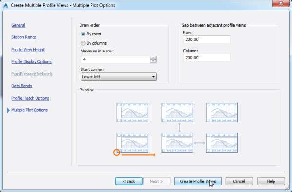
Figure 7.44 The Create Multiple Profile Views – Multiple Plot Options wizard page
- Click the Create Profile Views button and pick a point onscreen to create a view similar to Figure 7.45.

Figure 7.45 The staggered and gapped profile views of the RM2222 alignment
The gapped profile views are the four profile views on the bottom of the screen, and just like the staggered profile view, they show the entire alignment from start to finish. Unlike the staggered view, however, the gapped view is separated by a gap, creating four individual profile views. In addition, the gapped profile views are independent of each other, so they can be modified to have their own styles, properties, and labeling. This is also the primary way to create divided profile views for sheet production.
When this exercise is complete, you may save and close the drawing. A copy of the drawing at this stage is available from the book's web page with the filename 0709_GappedProfileView_FINISHED.dwg (0709_GappedProfileView_METRIC_FINISHED.dwg).
Creating Stacked Profile Views
In some parts of the United States, a three-line profile view is a common requirement. In this situation, the centerline is displayed in a central profile view, with left and right offsets shown in profile views above and below the centerline profile view. These are then typically used to show top-of-curb design profiles in addition to the centerline design. In this exercise, you look at how the Create Profile View Wizard makes generating these stacked views a simple process:
- Open the
0709_StackedProfileView.dwg(0709_StackedProfileView_METRIC.dwg) file. This drawing has sampled profiles for the RM2222 alignment at center as well as left and right offsets. - From the Home tab Profile & Section Views panel, choose Profile View Create Profile View to display the Create Profile View Wizard.
- Verify that the Select Alignment drop-down list shows RM2222, Profile Name is set to RM2222 Stacked Full Grid, and Full Grid is selected in the Profile View Style drop-down list.
- Check the Show Offset Profiles By Vertically Stacking Profile Views option on the General wizard page.
Notice that when you check this box, an additional link named Stacked Profile is added to the left sidebar of the wizard.
- Click Next.
- On the Create Profile View – Station Range wizard page, verify that Station Range is set to Automatic, and click Next.
- On the Create Profile View – Profile View Height wizard page, verify that Profile View Height is set to Automatic, and click Next.
- On the Create Profile View – Stacked Profile wizard page, set the gap between views to 15 (or 4 for metric users).
- Set the view styles to Top Stacked View, Middle Stacked View, and Bottom Stacked View, as shown in Figure 7.46. Click Next.
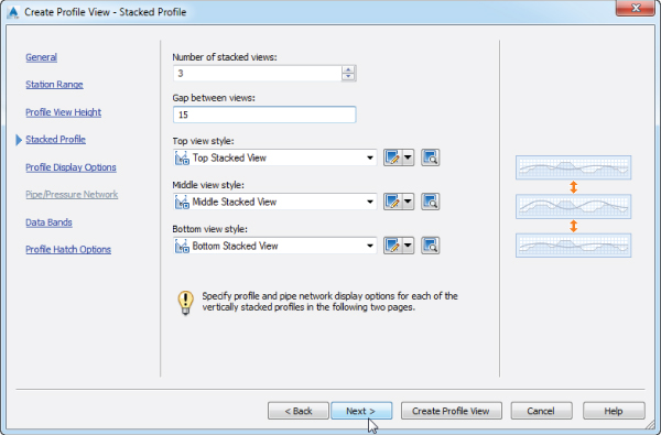
Figure 7.46 The Create Profile View – Stacked Profile wizard page
- On the Create Profile View – Profile Display Options wizard page, select Top View in the Select Stacked View To Specify Options For list box.
- Toggle the Draw option for the left offset profile (RM2222-EG - -30.000 (RM2222-EG - -10.000 for metric users)), as shown in Figure 7.47. If you need to widen the columns, you can do so by double-clicking the line between the column headings.
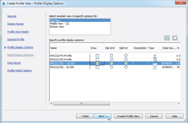
Figure 7.47 Setting the stacked view options for each view, in this case for the top view
Remember that the negative offset denotes a left profile whereas a positive offset denotes a right profile. You can also check the Offset column to verify the offset.
- Select Middle View - [1] in the Select Stacked View To Specify Options For list box.
- Toggle the Draw option for the sampled centerline profile (RM2222-EG-Profile) as well as the layout centerline profile (RM2222-FG-Profile).
- Select Bottom View in the Select Stacked View To Specify Options For list box.
- Toggle the Draw option for the right offset profile (RM2222-EG - 30.000 or RM2222-EG - 10.000 for metric users), and click Next.
- On the Data Bands wizard page, verify that the band set is set to EG-FG Elevations And Stations.
- Click the Create Profile View button and pick a point on the screen to draw the stacked profiles, as shown in Figure 7.48.
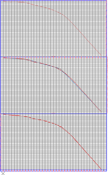
Figure 7.48 Completed stacked profiles
When this exercise is complete, you may save and close the drawing. A copy of the drawing at this stage is available from the book's web page with the filename 0709_StackedProfileView_FINISHED.dwg (0709_StackedProfileView_METRIC_FINISHED.dwg).
Like the gapped profile views that you generated in a previous exercise, the profile views are independent of one another, so they can be modified to have their own styles, properties, and labeling associated with them. The stacking here simply automates a process that many users previously found tedious. At this point you do not have finished grade information at the offsets, but you can add it to these views later by editing the Profile View Properties for those profile views.
When you create a profile, that profile will appear in any profile views that reference the same alignment. In the Profile View Properties dialog, you can always turn the Draw option off for any profile that should not appear in a given profile view.
Editing Profile Views
The profile view is one of the most sophisticated and flexible objects in the AutoCAD Civil 3D package. After a profile view is created, many modifications can be made to it without modifying the style or assigning a different style. In this series of exercises, you'll look at a number of changes that can be applied to any profile view in a given drawing.
Profile View Properties
Picking a profile view and then selecting Profile View Properties from the Profile View contextual tab ![]() Modify View panel yields the dialog shown in Figure 7.49. The properties of a profile include the style applied, station and elevation limits, the number of profiles displayed, the bands associated with the profile view, and any hatching that has been included. If a pipe network is displayed, a tab labeled Pipe Networks will appear. Also, if objects are projected in the profile view, then a Projections tab will be enabled and displayed as well. These tabs should look very similar to the links in the sidebar of the Create Profile View Wizard.
Modify View panel yields the dialog shown in Figure 7.49. The properties of a profile include the style applied, station and elevation limits, the number of profiles displayed, the bands associated with the profile view, and any hatching that has been included. If a pipe network is displayed, a tab labeled Pipe Networks will appear. Also, if objects are projected in the profile view, then a Projections tab will be enabled and displayed as well. These tabs should look very similar to the links in the sidebar of the Create Profile View Wizard.
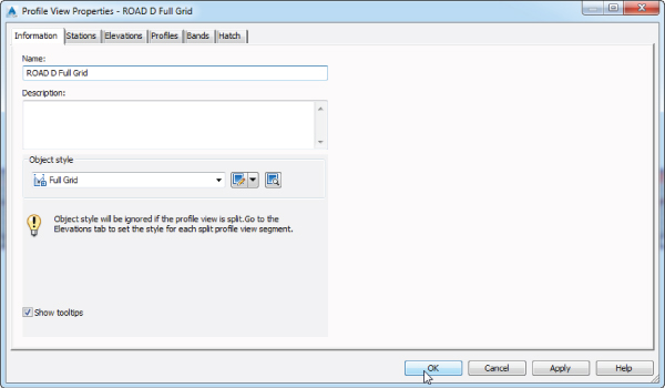
Figure 7.49 Typical Profile View Properties dialog
Adjusting the Profile View Station Limits
There are often times when a profile view needs to be manually adjusted. For example, the most common change is to limit the length of the profile view that is being shown so it fits on a specific size of paper or viewport. You can make some of these changes during the initial creation of a profile view (as shown in a previous exercise), but you can also make changes after the profile view has been created.
One way to do this is to use the Profile View Properties dialog to make changes to the profile view. The profile view is an AutoCAD Civil 3D object, so it has properties and styles that can be adjusted in this dialog to make the profile view look like you need it to.
- Open the
0710_ProfileViewProperties.dwg(0710_ProfileViewProperties_METRIC.dwg) file. - Zoom to the ROAD D Full Grid profile view.
- Pick a grid line, and from the Profile View contextual tab Modify View panel, choose the Profile View Properties icon button to display the Profile View Properties dialog.
- On the Stations tab, click the User Specified Range radio button, and set the value of the end station to 2200 (or 670 for metric users), as shown in Figure 7.50. Note that you do not need to type the + symbol.
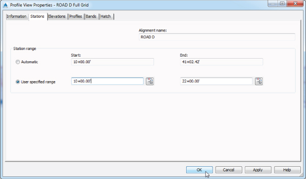
Figure 7.50 Adjusting the end station values for ROAD D
- Click OK to dismiss the dialog and press Esc to clear the selection.
The profile view will now reflect the updated end station value.
One of the nice things about Civil 3D is that copies of a profile view retain the properties of that view, making a gapped view easy to create manually if it was not created with the wizard.
- Press F8 on your keyboard to enable Ortho mode.
- Enter
Copy↵ on the command line. Pick the ROAD D Full Grid profile view you just modified. Make sure you are selecting the grid representing the profile view and not the linework that represents the profile. Press Enter to complete the selection. - Pick a base point and move the crosshairs to the right.
- When the crosshairs reach a point where the two profile views do not overlap, pick that as your second point, and press ↵ to end the
Copycommand. - Pick a grid line on the copy just created, and from the Profile View contextual tab Modify View panel, choose Profile View Properties to display the Profile View Properties dialog.
- On the Stations tab, set the Start field to 2200 (or 670 for metric users) and the End field to 4102.42 (or 1250.42 for metric users).
- Click OK to dismiss the dialog.
The total length of the alignment will now be displayed on the two profile views, with a gap between the two views at station 22+00 (or 0+760 for metric users).
You may want to move the copied profile view since it holds the station location, thus shifting it to the right. You could also copy the profile view in place and then change the settings, with no need to move the profile view.
Once this exercise is complete, your drawing will look like Figure 7.51.
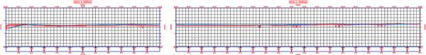
Figure 7.51 A manually created gap between profile views
You may save and close the drawing. A copy of the drawing at this stage is available from the book's web page with the filename 0710_ProfileViewProperties_FINISHED.dwg (0710_ProfileViewProperties_METRIC_FINISHED.dwg).
In addition to creating gapped profile views by changing the profile view properties, you could show phase limits by applying a different style to the profile in the second view.
Adjusting the Profile View Elevations
Another common issue is the need to control the height of the profile view. Civil 3D automatically sets the datum and the top elevation of profile views on the basis of the data to be displayed. In most cases this is adequate, but in others this simply creates a view too large for the space allocated on the sheet or does not provide the adequate room for layout PVIs to be placed.
- Open the
0710_ProfileViewElevations.dwg(0710_ProfileViewElevations_METRIC.dwg) file. - Zoom to the RM2222 Full Grid profile view, which is the first on the left.
- Pick a grid line, and from the Profile View contextual tab Modify View panel, choose Profile View Properties to display the Profile View Properties dialog.
- On the Elevations tab, in the Elevation Range section, check the User Specified Height radio button and set the maximum height to 1090 (or 332 for metric users), as shown in Figure 7.52.
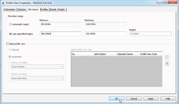
Figure 7.52 Modifying the height of the profile view
- Click OK to dismiss the dialog and press Esc to clear the selection.
The profile view of RM2222 should reflect the updated elevations, as shown in Figure 7.53.
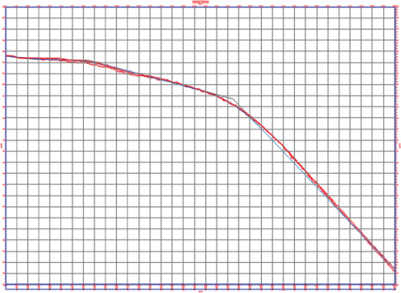
Figure 7.53 The updated profile view with the heights manually adjusted
The Elevations tab can also be used to split the profile view and create the staggered view that you previously created with the wizard.
- Pick the RM2222 Full Grid (1) profile view (the middle profile view).
- Pick a grid line, and from the Profile View contextual tab Modify View panel, choose Profile View Properties to display the Profile View Properties dialog.
- On the Profile View Properties dialog, switch to the Elevations tab.
- In the Elevations Range area, click the User Specified Height radio button.
- Check the Split Profile View option, and verify that the Automatic radio button is selected.
Notice that the Height field is now active.
- Set Height to 90 (or 26 for metric users), as shown in Figure 7.54.
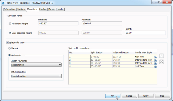
Figure 7.54 Defining a split profile view on the Elevations tab
- Click within the Split Profile View Data area to populate the splitting area, and click OK to exit the dialog.
- Enter
REGEN↵ on the command line.The profile view should look similar to Figure 7.55. If it doesn't, save and reopen the file and the desired layout will be displayed for the profile view.
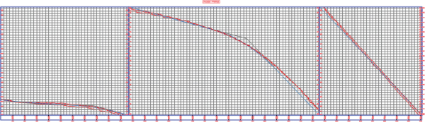
Figure 7.55 A split profile view for the RR2222 alignment
When this exercise is complete, save the drawing, but keep it open for the following exercise. A copy of the drawing at this stage is available from the book's web page with the filename 0710_ProfileViewElevations_FINISHED.dwg (0710_ProfileViewElevations_METRIC_FINISHED.dwg). Automatically creating split views is a good starting point, but you'll often have to tweak them as you've done here. The selection of the proper profile view styles is an important part of the Split Profile View process. We'll look at object styles in Chapter 19.
Using Profile Display Options
AutoCAD Civil 3D allows the creation of literally hundreds of profiles for any given alignment, which makes it easy to evaluate multiple design solutions, but it can also mean that profile views get very crowded. In this exercise, you'll look at some profile display options that allow the toggling of various profiles within a profile view:
- Continue using the file from the previous exercise, or open the
0710_ProfileViewElevations_FINISHED.dwg(0710_ProfileViewElevations_METRIC_FINISHED.dwg) file. - Click on the grid for the last profile view RM2222 Full Grid (1) (1).
- From the Profile View contextual tab Modify View panel, choose Profile View Properties to display the Profile View Properties dialog.
- Switch to the Profiles tab.
- Uncheck the Draw option for RM2222-FG-Profile and click OK. You might need to make the columns wider to be able to distinguish between the options.
Your profile view dialog settings should look similar to Figure 7.56.
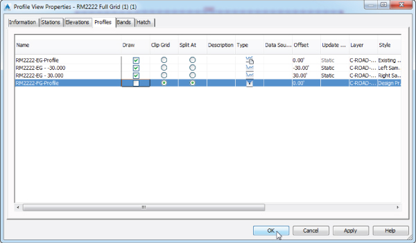
Figure 7.56 The RM2222 profile view settings with the Draw option toggled off for RM2222-FG-Profile
Toggling off the Draw option for the FG layout has created a profile view in which a profile of the desired design will not be drawn.
The FG profile still exists under the RM2222 alignment; it simply isn't shown in the current profile view.
When this exercise is complete, you may save and close the drawing. A copy of the drawing at this stage is available from the book's web page with the filename 0710_ProfileViewToggle_FINISHED.dwg (0710_ProfileViewToggle_METRIC_FINISHED.dwg).
Now that you've modified profile views using a number of methods, let's look at another option that is available on the Profile View Properties dialog: Profile View Bands.
Adding Profile View Bands
Data bands are horizontal elements that display additional graphical and numerical information about the profile or alignment that is referenced in a profile view. Bands can be applied to both the top and bottom of a profile view, and there are six different band types:
- Profile Data Bands Display information about the selected profile. This information can include simple elements such as elevation or more complicated information such as the cut-fill between two profiles at a given station.
- Vertical Geometry Bands Create a schematic view of the elements making up a profile. Typically used in reference to a design profile, vertical data bands make it easy for a designer to see the locations of tangents and vertical curves along an alignment as well as information about the tangents and vertical curves.
- Horizontal Geometry Bands Create a schematic view of the horizontal alignment elements, giving the designer or reviewer information about line, curve, and spiral segments and their relative location to the profile data being displayed.
- Superelevation Data Bands Display the various options for superelevation values at the critical points along the alignment.
- Sectional Data Bands Can display information about the sample line locations and the distance between them as well as other section-related information.
- Pipe Network Bands Can display specific information such as part, offset, elevation, or direction about each pipe or structure being shown in the profile view.
In this exercise, you'll add bands to give feedback on the EG and layout profiles as well as horizontal and vertical geometry:
- Open the
0711_ProfileViewBands.dwg(0711_ProfileViewBands_METRIC.dwg) file. - Zoom to the ROAD D Full Grid profile view.
- Pick a grid line, and from the Profile View contextual tab Modify View panel, choose Profile View Properties to display the Profile View Properties dialog.
- On the Bands tab (Figure 7.57), in the List Of Bands area, verify that the Location drop-down is set to Bottom Of Profile View and notice that an Elevations And Stations band has already been set during the creation of this profile view.
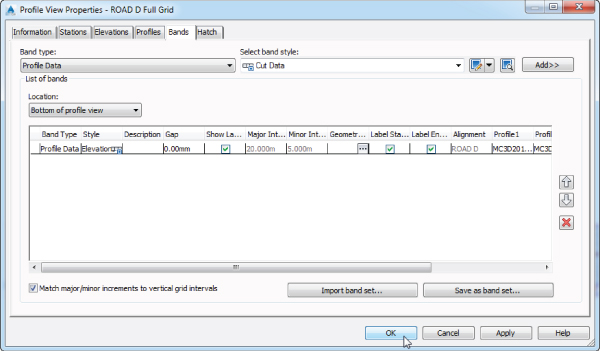
Figure 7.57 The Bands tab of the Profile View Properties dialog
Selecting the type of band from the Band Type drop-down menu changes the Select Band Style drop-down menu so that it includes only styles that are available for the band type you select. Next to the Select Band Style drop-down menu are the usual Style Edit/Copy button and a preview button. Once you've selected a style from the Select Band Style drop-down, clicking the Add button places it on the profile. The Location drop-down list in the List Of Bands section of this dialog allows you to switch between the bands shown at the bottom of the profile view or the top of the profile view; you'll look at that in a moment.
- Change the Band Type drop-down to the Profile Data option and choose the Cut Data option from the Select Band Style drop-down.
- Click the Add button. The Geometry Points To Label In Band dialog will open (Figure 7.58).
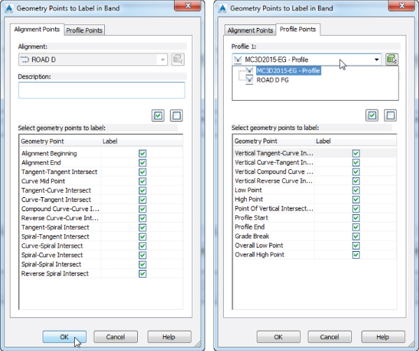
Figure 7.58 The Geometry Points To Label In Band dialog showing the Alignment Points tab (left) and the Profile Points tab (right)
- Click OK to accept the defaults in the Geometry Points To Label In Band dialog.
- Leave Band Type set to Profile Data, and choose the Fill Data option from the Select Band Style drop-down.
- Click the Add button, which will open the Geometry Points To Label In Band dialog once again. Click OK to accept the defaults and dismiss that dialog.
- Change the Location drop-down to Top Of Profile View.
- Change the Band Type drop-down to the Horizontal Geometry option and choose the Geometry option from the Select Band Style drop-down.
- Click the Add button to add the Horizontal Geometry band to the table in the List Of Bands area.
- Change the Band Type drop-down to the Vertical Geometry option.
Do not change the Select Band Style field from its current selection (Geometry).
- Click the Add button to also add the Vertical Geometry band to the table in the List Of Bands area.
- Click OK to exit the dialog and press Esc to deselect.
Your profile view should look like Figure 7.59.

Figure 7.59 Applying bands to a profile view
There are obviously problems with the bands. The Vertical Geometry band is a mess and is located above the title of the profile view, whereas the Horizontal Geometry band overwrites the title. In addition, the elevation information has only the existing ground profile being referenced. Next, you'll fix those issues.
- Pick a grid line on ROAD D Full Grid profile view.
- From the Profile View contextual tab Modify View panel, choose Profile View Properties to display the Profile View Properties dialog.
- On the Bands tab, verify that the Location drop-down in the List Of Bands area is set to Bottom Of Profile View.
- Verify that the Match Major/Minor Increments To Vertical Grid Intervals option at the bottom of the page is selected.
Checking this option ensures that the major/minor intervals of the profile data band match the major/minor profile view style's major/minor grid spacing.
Three Profile Data bands are listed in the table in the List Of Bands area (Elevations And Stations, Cut Data, and Fill Data). If you need to widen the columns, you can do so by double-clicking the line between the column headings.
- Scroll right and notice the two columns labeled Profile1 and Profile2.
- For all three rows change the value of Profile2 to ROAD D FG, as shown in Figure 7.60.
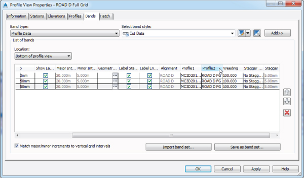
Figure 7.60 Setting the profile view bands to reference the ROAD D FG profile
- Change the Location drop-down to Top Of Profile View.
The Horizontal Geometry and Vertical Geometry bands are now listed in the table.
- Scroll to the right again, and set the value of Profile1 in the Vertical Geometry band to ROAD D FG.
Notice that some of the Profile1 and Profile2 boxes are not available for editing, such as those in the horizontal geometry band in the Top Of Profile View; this is because profile information isn't needed for this band.
- Scroll back to the left and set the Gap value for the Horizontal Geometry band and the one for the Vertical Geometry band to 2” (or 35 mm for metric users).
This value controls the distance from one band to the next for all bands for both top and bottom locations, except the first in the list of bands, for which this value defines the offset of the band from the bottom or top of the profile view, respectively.
- Click OK to dismiss the dialog.
Your profile view should now look like Figure 7.61.
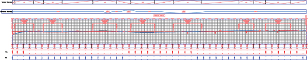
Figure 7.61 Completed profile view with the bands appropriately spaced
You may save and close the drawing. A finished copy of this is available from the book's web page with the filename 0711_ProfileViewBands_FINISHED.dwg (0711_ProfileViewBands_METRIC_FINISHED.dwg).
Bands use the Profile1 and Profile2 designation as part of their style construction. By changing the profile referenced as Profile1 or Profile2, you change the values that are calculated and displayed (e.g., existing versus proposed elevations). These bands are just additional items that are driven by object styles, which you will learn more about in Chapter 19.
In the next section we'll look at using band sets to make working with bands more efficient.
Band Sets
Band sets are simply collections of bands, much like the profile label sets or alignment label sets. In this exercise, you'll save a band set and then apply it to a second profile view:
- Open the
0711_ProfileViewBandsSet.dwg(0711_ProfileViewBandsSet_METRIC.dwg) file. - Pick a grid line in the ROAD D Full Grid profile view (the top profile view), and from the Profile View contextual tab Modify View panel, choose Profile View Properties to display the Profile View Properties dialog.
- On the Bands tab, click the Save As Band Set button to display the Band Set – New Profile View Band Set dialog.
- On the Information tab, in the Name field, enter Cut Fill Elev Station and Horiz Vert Geometry, as shown in Figure 7.62.
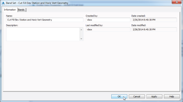
Figure 7.62 The Information tab for the Band Set – New Profile View Band Set dialog
- Click OK to dismiss the Band Set – New Profile View Band Set dialog.
- Click OK to dismiss the Profile View Properties dialog.
- Press Esc to clear your selection, then pick a grid line in the ROAD A Full Grid profile view (profile view on the bottom), and from the Profile View contextual tab Modify View panel, choose Profile View Properties to display the Profile View Properties dialog.
- On the Bands tab, click the Import Band Set button, and the Band Set dialog opens.
- Select the Cut Fill Elev Station And Horiz Vert Geometry option from the drop-down list and click OK.
- Select Top Of Profile View from the Location drop-down list.
- Scroll over on the Vertical Geometry row and set Profile1 to ROAD A FG.
- Select Bottom Of Profile View from the Location drop-down list.
- Scroll over and change Profile2 to ROAD A FG for all three rows. Also make sure that Profile1 is set to MC3D2015-EG for all three as well.
- Click OK to exit the Profile View Properties dialog.
Your ROAD A Full Grid profile view (Figure 7.63) now looks like the ROAD D Full Grid profile view with the exception of the finished grade labels.
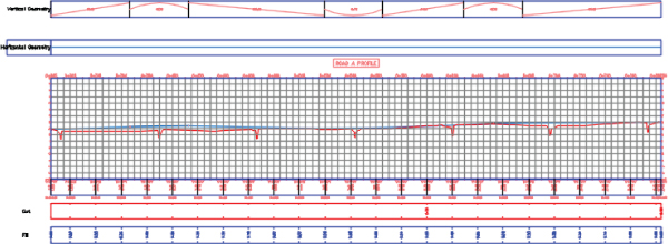
Figure 7.63 Completed profile view after importing the band set and assigning profiles
Band sets allow you to create uniform labeling and callout information across a variety of profile views. By using a band set, you can take a collection of settings and styles that you've assigned to a single profile view and apply them to a number of profile views. The simplicity of enforcing standard profile view labels and styles makes using profiles and profile views simpler than ever.
You may save and close the drawing. A finished copy of this drawing is available from the book's web page with the filename 0711_ProfileViewBandsSet_FINISHED.dwg (0711_ProfileViewBandsSet_METRIC_FINISHED.dwg).
Understanding Profile View Hatch
Sometimes it is necessary to hatch cut/fill areas in a profile view. The settings on the Hatch tab of the Profile View Properties dialog are used to specify upper and lower cut/fill boundary limits for associated profiles (see Figure 7.64).
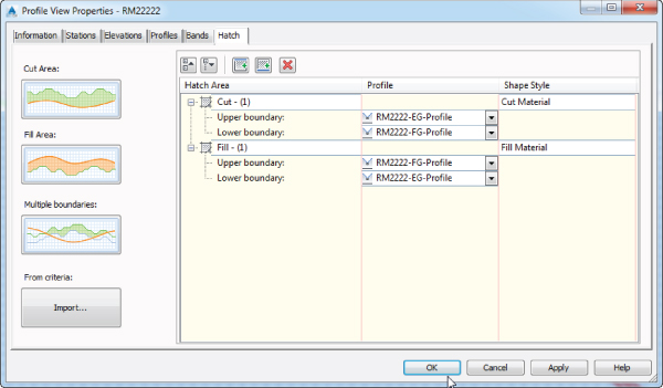
Figure 7.64 Shape style selection on the Hatch tab of the Profile View Properties dialog
Shape styles from the General Multipurpose Styles collection found on the Settings tab of Toolspace can also be selected here. These settings include the following:
- Cut Area Click this button to add hatching to a profile view in areas of cut (the layout profile is at a lower elevation than the sampled surface profile).
- Fill Area Click this button to add hatching to a profile view in areas of fill (the layout profile is at a higher elevation than the sampled surface profile).
- Multiple Boundaries Click this button to add hatching to a profile view in areas of a cut/fill where the area must be averaged between two existing profiles (for example, finished ground at the centerline vs. the left and right top of a curb).
- From Criteria Click this button to add hatch in areas where quantity takeoff criteria are used to define a hatch region.
Figure 7.65 shows a cut and fill hatched profile based on the criteria shown previously in Figure 7.64.
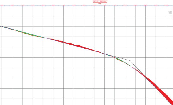
Figure 7.65 A portion of the RM2222 profile shown with cut and fill shading
Mastering Profiles and Profile Views
One of the most difficult concepts to master in AutoCAD Civil 3D is the notion of which settings control which display property. Although the following two rules may sound overly simplistic, they are important to remember and will help you work through your understanding of the software:
- Every object has a label and an object style.
- Every label has a label style.
Furthermore, if you can remember that there is a distinct difference between a profile object and the profile view object you place it in, you'll be well on your way to mastering profiles and profile views. When in doubt, select an object and observe the options that become available on the contextual ribbon tab. Label styles and object styles will be discussed further in Chapters 18 and 19, respectively.
Profile View Labeling Styles
Now that the profile view is created, the profile view grid spacing is set, and the titles all look good, it's time to add some specific callouts and detail information. Civil 3D uses profile view labels and bands for annotating. The specific label styles will be discussed further in Chapter 18, but for now we will just discuss how to apply the labels.
View Annotation
Profile view annotations label individual points in a profile view, but they are not tied to a specific profile object. Profile view labels can be station elevation labels, depth labels, or projection labels. Station elevation labels can be used to label a single point or the depth between two points in a profile while recognizing the vertical exaggeration of the profile view and applying the scaling factor to label the correct depth. In this exercise, you'll use both the station elevation label and the depth label:
- Open the
0712_ProfileViewLabels.dwg(0712_ProfileViewLabels_METRIC.dwg) file. - Zoom to the ROAD D Full Grid profile view.
- From the Annotate tab Labels & Tables panel, choose Add Labels (not the drop-down list) to open the Add Labels dialog.
- In the Feature drop-down, select Profile View.
- In the Label Type drop-down, verify that Station Elevation is selected.
- In the Station Elevation Label Style drop-down, verify that Station And Elevation is selected.
- Verify that the marker style is set to Basic Circle With Cross.
- Click the Add button.
- When prompted to select a profile view, click a grid line in the ROAD D Full Grid profile view, and a vertical red line will appear.
- Zoom in around station 11+40 (or 0+347 for metric users) so that you can see the point where the EG and layout profiles cross.
- Turn off your running Osnaps and pick this profile crossover point visually; then pick the same point to set the elevation and press ↵.
Your label should look like Figure 7.66, although the actual values will vary slightly.
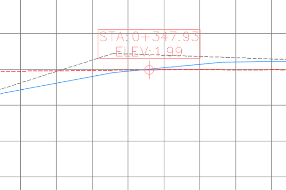
Figure 7.66 A profile view station and elevation label
- In the Add Labels dialog, change both Label Type and Depth Label Style to the Depth option.
- Click the Add button.
- Pick the ROAD D Full Grid profile view by clicking one of the grid lines.
- Pick a point along the layout profile; then pick a point along the EG profile and press ↵.
The depth between the two profiles will be measured, as shown in Figure 7.67. Your value may vary slightly from what is shown.
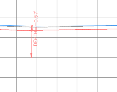
Figure 7.67 A depth label applied to the ROAD D Full Grid profile view
- Close the Add Labels dialog.
You may save and close the drawing. A finished copy of this drawing is available from the book's web page with the filename 0712_ProfileViewLabels_FINISHED.dwg (0712_ProfileViewLabels_METRIC_FINISHED.dwg).
Depth labels can be handy in earthworks situations where cut and fill become critical, and individual spot labels are important to understanding points of interest, but most design documentation is accomplished with labels placed along the profile view axes in the form of data bands and band sets discussed earlier in this chapter.
Profile Labels
It's important to remember that the profile and the profile view aren't the same thing. The labels discussed in the following sections are those that relate directly to the profile but are visible for a specific profile view. This usually means station-based labels, individual tangent and curve labels, or grade breaks.
Applying Labels
As with alignments, you can apply labels as a group of objects separate from the profile. In this portion of the exercise, you'll learn how to add labels along a profile object:
- Open the
0712_ProfileLabels.dwg(0712_ProfileLabels_METRIC.dwg) file. - Zoom to the ROAD D Full Grid profile view and pick the ROAD D FG profile (the blue line) to activate the Profile contextual tab.
 From the Profile contextual tab Labels panel, choose Edit Profile Labels to display the Profile Labels dialog (see Figure 7.68).
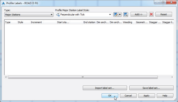
Figure 7.68 An empty Profile Labels dialog
Selecting the type of label from the Type drop-down menu changes the Style drop-down menu to include styles that are available for that label type. Next to the Style drop-down menu are the usual Style Edit/Copy button and Preview button. Once you've selected a style from the Style drop-down menu, clicking the Add button places it on the profile. The middle portion of this dialog displays information about the labels that are being applied to the profile selected; you'll look at that in a moment.
- Choose the Major Stations option from the Type drop-down menu.
The name of the second drop-down menu changes to Profile Major Station Label Style to reflect this option.
- Verify that Perpendicular With Tick is selected in this menu.
- Click the Add button to apply this label to the profile.
- Choose Horizontal Geometry Points from the Type drop-down menu.
The name of the Style drop-down menu changes to Profile Horizontal Geometry Point.
- Select the Horizontal Geometry Station option, and click the Add button again to display the Geometry Points dialog.
This dialog lets you apply different label styles to different geometry points if necessary.
- Deselect the Alignment Beginning and Alignment End rows, as shown in Figure 7.69, and click OK to dismiss the dialog.
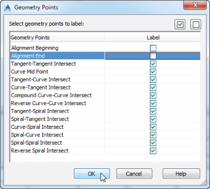
Figure 7.69 The Geometry Points dialog appears when you apply labels to horizontal geometry points.
- On the Profile Labels dialog, click the Apply button.
- Drag the dialog out of the way to view the changes to the profile, as shown in Figure 7.70.
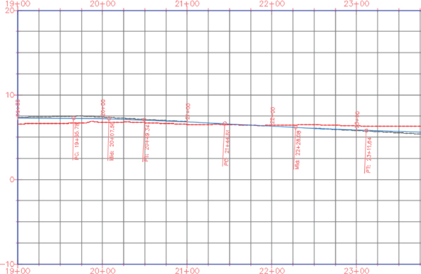
Figure 7.70 Labels applied to major stations and alignment geometry points
- In the middle of the Profile Labels dialog, change the Increment value in the Major Stations row to 50 (or 10 for metric users), as shown in Figure 7.71.
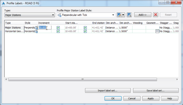
Figure 7.71 Modifying the major station labeling increment
This modifies the labeling increment only, not the grid or other values.
- Click OK to dismiss the Profile Labels dialog.
You may save and close the drawing. A finished copy of this drawing is available from the book's web page with the filename 0712_ProfileLabels_FINISHED.dwg (0712_ProfileLabels_METRIC_FINISHED.dwg).
Using Profile Label Sets
Applying labels to both crest and sag curves and to tangents, grade breaks, and geometry with the label style selection and various options can be monotonous. Thankfully, Civil 3D gives you the ability to use label sets, as in alignments, to make the process quick and easy. Just as you saved and imported band sets in a previous example, you can save and import label sets as well.
In all of the previous examples, you used either the complete label set or the _No Labels label set, which you specified on the Profile Display Options wizard page.
Label sets are the best way to apply profile labeling uniformly. When you're working with a well-developed set of styles and label sets, it's quick and easy to go from sketched profile layout to plan-ready output. We will discuss profile label sets in further detail and go over an example in Chapter 18.
Profile Utilities
One common requirement is to compare profile data for objects that are aligned similarly but not parallel. Another is the ability to project objects from a plan view into a profile view. The abilities to superimpose profiles and project objects are both discussed in this section.
Superimposing Profiles
In a profile view, a profile is sometimes superimposed to show one profile adjacent to another (e.g., a ditch adjacent to a road centerline). In this brief exercise, you'll superimpose one of your street designs onto the other to see how they compare over a certain portion of their length:
- Open the
0713_SuperImposeProfile.dwg(0713_SuperImposeProfile_METRIC.dwg) file.  From the Home tab Create Design panel, choose Profile Create Superimposed Profile.
- At the
Select source profile:prompt, zoom to the ROAD C TRAIL Full Grid profile view and pick the ROAD C TRAIL FG profile (the blue line). - At the
Select destination profile view:prompt, click one of the grid lines in the ROAD C Full Grid profile view to display the Superimpose Profile Options dialog shown in Figure 7.72.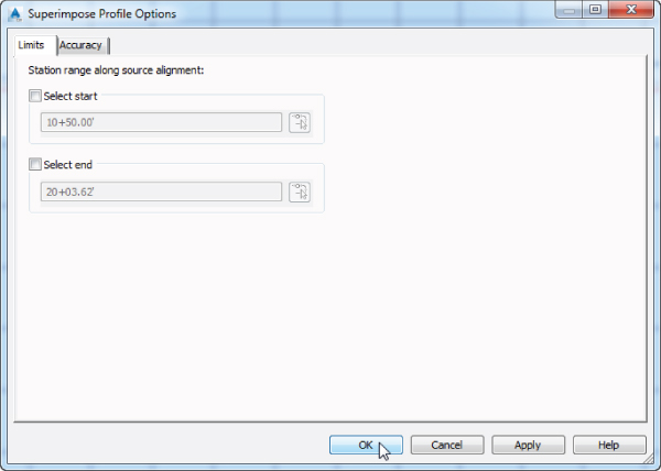
Figure 7.72 The Superimpose Profile Options dialog
On the Limits tab you can control the start and end stations of the superimposed profile, in the event that you do not want the entire profile to be superimposed. On the Accuracy tab, you can control the handling of curves through the mid-ordinate settings. Superimposed curves aren't curves at all; they are lots of small segments that approximate a curve. The smaller the mid-ordinate distance values, the smaller and more numerous the segments will be.
- Click OK to dismiss the dialog, accepting the default settings.
- Zoom in on the ROAD C Full Grid profile view to see the superimposed data, as shown in Figure 7.73.
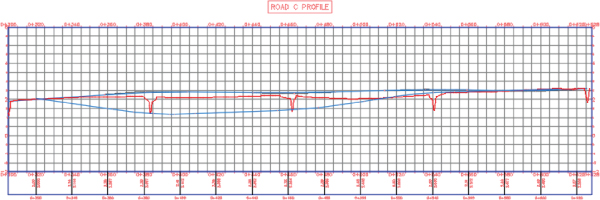
Figure 7.73 The ROAD C TRAIL FG layout profile superimposed on the ROAD C Full Grid profile view
Note that the vertical curves in the ROAD C TRAIL FG layout profile have been approximated on the ROAD C Full Grid profile view, using a series of PVIs. Superimposing works by projecting a line from the target alignment (ROAD C) to a perpendicular intersection with the other source alignment (ROAD C TRAIL).
The target alignment is queried for an elevation at the intersecting station, and a PVI is added to the superimposed profile. Note that this superimposed profile is still dynamic! A change in the ROAD C TRAIL FG layout profile will be reflected on the ROAD C Full Grid profile view.
When this exercise is complete, you may save and close the drawing. A finished copy of this drawing is available from the book's web page with the filename 0713_SuperImposeProfile_FINISHED.dwg (0713_SuperImposeProfile_METRIC_FINISHED.dwg).
Projecting Objects in Profile View
Some AutoCAD and some AutoCAD Civil 3D objects can be projected from a plan view into a profile view. The list of available AutoCAD objects includes points, blocks, 3D solids, and 3D polylines. The list of available AutoCAD Civil 3D objects includes COGO points, feature lines, and survey figures. These objects can be projected to the object's elevation, a manually selected elevation, a surface, or a profile. In the following exercise, you'll project a 3D object into a profile view:
- Open the
0714_ProjectToProfile.dwg(0714_ProjectToProfile_METRIC.dwg) file.  From the Home tab Profile & Section Views panel, choose Profile View Project Objects To Profile View.
- At the
Select objects to add to profile view:prompt, select the three power poles and the fire hydrant object located along the left and right of the ROAD C alignment and press ↵. - At the
Select a profile view:prompt, select the ROAD C Full Grid profile view by clicking one of the grid lines to display the Project Objects To Profile View dialog. - Verify that Style is set to Power Pole for the power poles object and to Hydrant (existing) for the hydrant object, Elevation Options is set to Surface MC3D2015-EG, and Label Style is set to Projection Dimension Below, as shown in Figure 7.74.
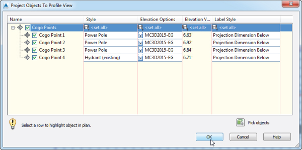
Figure 7.74 A completed Project Objects To Profile View dialog
- Click OK to dismiss the dialog, and review your results, as shown in Figure 7.75.
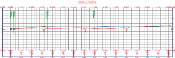
Figure 7.75 The COGO point objects projected into a profile view
We actually wanted the second power pole along the alignment to show on the proposed surface. No problem. Follow the next steps.
- Click the power pole in profile view to activate the Cogo Point contextual tab. Together with this tab another tab is activated, the Projected Object tab. Switch to this contextual tab.
 From the Projected Object contextual tab Modify Projected Object panel, choose Projection Properties to display the Profile View Properties dialog.
- In the Profile View Properties dialog, click the cell in the Elevation Options column for the Cogo Point 2 object, and from the drop-down select Profile ROAD C FG, as shown in Figure 7.76. Click OK.
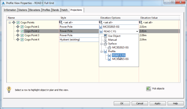
Figure 7.76 Selecting the ROAD C FG profile elevation
The projected power pole is now adjusted to match the elevation of the ROAD C FG profile, as shown in Figure 7.77.

Figure 7.77 The COGO point object projected onto the ROAD C FG profile
You may save and close the drawing. A finished copy of this drawing is available from the book's web page with the filename 0714_ProjectToProfile_FINISHED.dwg (0714_ProjectToProfile_METRIC_FINISHED.dwg).
Once an object has been projected into a profile view, the Profile View Properties dialog will display a new Projections tab. Projected objects will remain dynamically linked with respect to their plan placement. If you move them manually after placing them dynamically, a warning will appear to confirm that you want to break the dynamic setting. Because profile views and section views are similar in nature, objects can be projected into section views in the same fashion. However, projecting a feature line onto a profile view will give you a different result than projecting it onto a section view. On a profile view, it looks more like a superimposed profile. On a section view, it's more like a pipe crossing since it appears only where it intersects the section line.
Creating a Quick Profile
There are going to be times when all you want is to quickly look at a profile and not keep it for later use. When this is the case, instead of creating an alignment, a profile, and a profile view, you can create a quick profile. A quick profile is a temporary object that will not be saved with the drawing. You can create a quick profile for 2D or 3D lines or polylines, lot lines, feature lines, survey figures, and even a series of points.
From the Home tab ![]() Create Design panel, choose Profile
Create Design panel, choose Profile ![]() Quick Profile. The command line will state
Quick Profile. The command line will state Select object or [by Points]:. Once you select your object (or points), the Create Quick Profiles dialog is displayed (Figure 7.78).
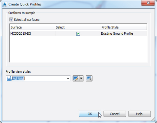
Figure 7.78 The Create Quick Profiles dialog
You can select which surface you want to sample as well as what profile view style and 3D entity profile style to use. Upon clicking OK, you will be prompted for a location to place the profile. A quick profile is a temporary profile that will be erased once a user save operation is performed on the drawing. You cannot select a different style to use for this profile view and cannot sample other sources once the profile view is created. Also, you will not be able to use the profile layout tools to define a design profile on this type of profile view.
The Bottom Line
- Sample a surface profile with offset samples. Using surface data to create dynamic sampled profiles is an important advantage of working with a three-dimensional model. Quick viewing of various surface centerlines and grip-editing alignments makes for an effective preliminary planning tool. Combined with offset data to meet review agency requirements, profiles are robust design tools in Civil 3D.
- Master It Open the
MasterIt_0701.dwg(MasterIt_0701_METRIC.dwg) file and sample the ground surface along Alignment A, along with offset values at 15′ left and 15′ right (or 4.5 m left and 4.5 m right) of the alignment. Generate a profile view showing this information using the Major Grids profile view style with no data band sets.
- Master It Open the
- Lay out a design profile on the basis of a table of data. Many programs and designers work by creating pairs of station and elevation data. The tools built into Civil 3D let you input this data precisely and quickly.
- Master It Continue in the previous file or open
MasterIt_0701_FINISHED.dwg(MasterIt_0701_METRIC_FINISHED.dwg). Create a layout profile on Alignment A using the Layout profile style and a complete label set with the following information for Imperial users.Station PVI Elevation Curve Length 0+00 822.00 1+80 825.60 300′ 6+50 800.80
Or use the following information for metric users:
Station PVI Elevation Curve Length 0+000 250.400 0+062 251.640 100 m 0+250 244.840 - Master It Continue in the previous file or open
- Add and modify individual entities in a design profile. The ability to delete, modify, and edit the individual components of a design profile while maintaining the relationships is an important concept in the 3D modeling world. Tweaking the design allows you to pursue a better solution, not just a working solution.
- Master It Continue in the previous file or open
MasterIt_0702_FINISHED.dwg(MasterIt_0702_METRIC_FINISHED.dwg). For the layout profile created in the previous exercise, modify the curve so that it is 200′ (or 60 m for metric users). Then insert a PVI at Station 4+90, Elevation 794.60 (or at Station 0+150, Elevation 242.840 for metric users) and add a 300′ (or 96 m for metric users) parabolic vertical curve at the newly created PVI.
- Master It Continue in the previous file or open
- Apply a standard band set. Standardization of appearance is one of the major benefits of using styles in labeling. By applying band sets, you can quickly create plot-ready profile views that have the required information for review.
- Master It Continue in the previous file or open
MasterIt_0703_FINISHED.dwg(MasterIt_0703_METRIC_FINISHED.dwg). Apply the Cut And Fill band set to the layout profile created in the previous exercise with the appropriate profiles referenced in each of the bands.
- Master It Continue in the previous file or open