
Chapter 10
Advanced Corridors, Intersections, and Roundabouts
This chapter focuses on taking your corridor-modeling skills to a new level by introducing more tools to your corridor-building toolbox, such as intersecting roads, cul-de-sacs, advanced techniques, and troubleshooting. You will use advanced corridor targets and work with conditional subassemblies.
This chapter assumes that you've worked through the examples in the chapters on alignments, profiles, profile views, assemblies, and basic corridors. Without a strong knowledge of the foundational skills, many of the tasks in this chapter will be difficult.
In this chapter, you will learn to
- Create corridors with non-centerline baselines
- Add alignment and profile targets to a region for a cul-de-sac
- Create a surface from a corridor and add a boundary
Using Multiregion Baselines
In the previous chapter, you modeled corridors with one baseline and one region. A question many people ask when working with corridors is, “At what point do I need another region?” The answer is simple: If you need a different assembly, you need a different region.
In the following example, you will step through adding an additional region to an existing baseline:
- Open the drawing
1001_MultiRegionCorr.dwg(1001_MultiRegionCorr_METRIC.dwg), which you can download from this book's web page, www.sybex.com/go/masteringcivil3d2015.This drawing has been split into two modelspace viewports so that you can observe the results of your efforts in 3D.
- Select the corridor and, from the Corridor contextual tab
 Modify Corridor panel, select Corridor Properties.
On the Parameters tab of the Corridor Properties dialog, notice that there is a baseline containing a single region.
- Click the icon in the End Station column for the region to pick a new end station in the drawing, as shown in Figure 10.1.
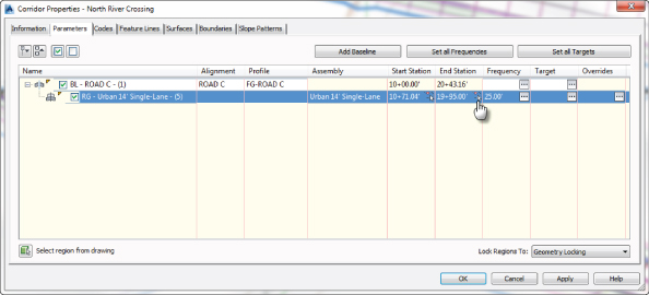
Figure 10.1 Changing the region end station
The Corridor Properties dialog temporarily disappears. The drawing contains linework representing the edge of pavement for this network of roadways in this subdivision. You will be using your Endpoint Osnap along with this linework to define multiple regions in this corridor.
- In the drawing, with your cursor anchored to ROAD C, stretch the station picker south and Osnap to the end point of the left arc where it intersects ROAD C's edge of pavement, as shown in Figure 10.2.
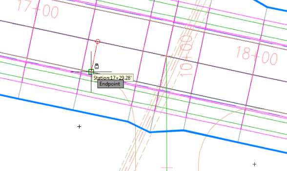
Figure 10.2 Using Osnaps to help define regions
The Corridor Properties dialog reappears. Notice the new End Station value.
- Click Apply, and rebuild the corridor if prompted.
- Move the Corridor Properties dialog aside to review the corridor in the drawing area.
Notice that the corridor region now stops exactly at the beginning of the curb return; you would not want the curb and gutter, sidewalk, and daylighting to shoot through the intersection on the right side of the road. In this situation you need another assembly, one without curb and gutter on the right. Since it is needed only in the intersection area, you'll add a region that picks up where the first region left off and ends at the end point of the opposite curb return.
- Right-click the region and select Insert Region - After.
- In the Create Corridor Region dialog, using the drop-down menu under Assembly, select Left Daylight-Right Pavement, as shown in Figure 10.3.
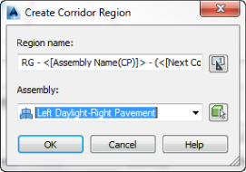
Figure 10.3 Assigning an assembly after inserting a new region
- Click OK to close the Create Corridor Region dialog.
- Click the ellipsis button in the Target column of the new region to open the Target Mapping dialog.
This assembly contains a daylighting subassembly, so you'll need to set the surface target.
- In the Object Name column next to Target Surface, click <None> to open the Pick A Surface dialog.
- Select Existing Surface and click OK to close.
- Click OK to close the Target Mapping dialog.
- Click OK to close Corridor Properties and rebuild the corridor if prompted.
The new region was added but it is extending to the end of ROAD C, which wasn't the intent. Next, you will split that region in two and assign another assembly to finish this part of the corridor.
- Select the corridor and open Corridor Properties using the contextual ribbon.
- On the Parameters tab, right-click the second region and select Split Region.
- Use your Endpoint Osnap to select the point where the curb return on the opposite side of the road meets the edge of pavement of ROAD C. Press ↵.
If you see a warning dialog referring to 0+00 being outside of the station limits, click OK and continue.
Back on the Parameters tab, you now have three regions listed under your baseline. The last region requires an assembly change since this is the section on the corridor that requires curb and gutter, sidewalk, and daylighting on both sides.
- On the third region in the Assembly column, click to open the Edit Corridor Region dialog. Using the drop-down menu under Assembly, select Full Section.
- Set the surface targets for both sides of the road as described in steps 10–13.
- Change the end station for the third region to 1995 (608 for metric).
- Click OK to close Corridor Properties and rebuild the corridor if prompted.
The corridor along ROAD C is nearly complete with the exception of the curb returns, as shown in Figure 10.4.
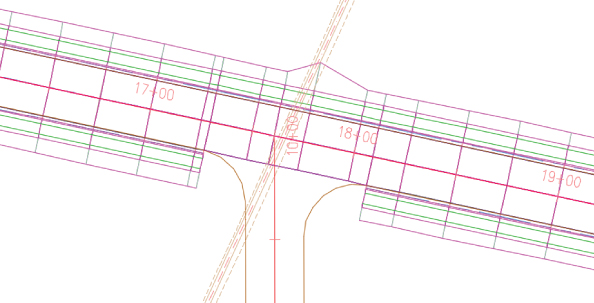
Figure 10.4 Corridor with multiple-baselines
The files
1001_MultiRegionCorr_FINISHED.dwgand1001_MultiRegionCorr_METRIC_FINISHED.dwgare available on this book's web page for you to check your work.
Instead of moving into building out the regions required for the curb returns, you're going to switch gears for a bit and look at a building a cul-de-sac region. Then after you build the cul-de-sac, you'll learn how to use the intersection tool, which automates the process of creating regions, assigning assemblies, and designating targets.
Modeling a Cul-de-Sac
Even if you never plan to design one in real life, understanding what is going on in a cul-de-sac corridor model will set you on the right path for building more complex models. If you truly understand the principles explained in the section that follows, then expanding your repertoire to include intersections and roundabouts will become much easier.
Using Multiple Baselines
Up to this point, every corridor you've built has had a single baseline. When you worked with corridor surfaces, you were working with a complex corridor with multiple baselines. A cul-de-sac by itself can be modeled in two baselines, as shown in Figure 10.5. The procedures that follow will work for most cul-de-sacs, including symmetrical, asymmetrical, and hammerhead styles. You will need a centerline alignment and design profile for the road leading into the cul-de-sac as well as an edge of pavement (EOP) alignment and design profile defining the cul-de-sac bulb.
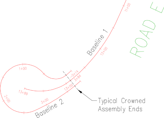
Figure 10.5 Example cul-de-sac alignment setup
In the example shown in Figure 10.5, the centerline of the road, Baseline 1, will require a typical crowned assembly, which will terminate when it reaches the point in the cul-de-sac geometry where the bulb defining curvature begins. From that point, the baseline is swapped out for an alignment and profile that define the edge of the cul-de-sac.
As you've seen, when assemblies are applied to a baseline, the geometry of the subassemblies project perpendicularly from the baseline. In the example of Figure 10.5, the curb and gutter subassembly as well as the rest of the subassemblies it carries (sidewalk, daylighting) need to be projected from the edge of the cul-de-sac bulb because that's the way their real-life counterparts are built. The assembly used on this baseline will have the curb and gutter subassembly on one side and the lane subassembly on the opposite side (Figure 10.6). The lane subassembly will stretch to meet the centerline alignment and profile as its targets.
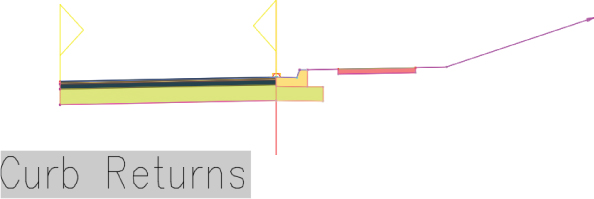
Figure 10.6 Assembly used for designing off the edge of pavement
It helps to think of the assembly as radiating away from the baseline, from the assembly base outward, toward a target (Figure 10.7). Because the assemblies are applied to the baseline in a perpendicular manner, using the edge of pavement for a baseline in curved areas (such as cul-de-sac bulbs or curb returns) will result in a smooth, properly graded pavement surface.
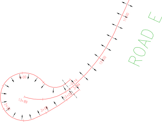
Figure 10.7 It helps to think of the assemblies radiating away from the baseline toward the targets.
Establishing EOP Design Profiles
One of the most challenging parts of complex corridor (i.e., cul-de-sac, intersection, or roundabout) is establishing design profiles for non-centerline alignments. You must have design profiles for both the centerline and edge of pavement alignments, but it does not have to be a painful process to obtain them.
Using a simple, preliminary corridor and the profile-creation tools you learned about in Chapter 7, “Profiles and Profile Views,” you'll find that establishing an edge of pavement profile can go quickly.
In the exercise that follows, you will work through the steps of creating an EOP profile:
- Open the
1002_EOPProfile.dwg(1002_EOPProfile_METRIC.dwg) file, which you can download from this book's web page, www.sybex.com/go/masteringcivil3d2015.This drawing contains the corridor you worked on in the last exercise, plus an additional baseline and region built for ROAD E. You may also notice that there is an alignment tracing around what would be the edge of pavement in the cul-de-sac for ROAD E.
- Click the corridor, and open Corridor Properties from the contextual ribbon.
- On the Surfaces tab of Corridor Properties, do the following:
-
 Click the Create A Corridor Surface button.
- Rename the surface to North River Crossing - Top.
- Change the surface style to Border Only.
- Under Add Data, verify that the Data Type setting is set to Links and the Specify Code setting is set to Top.
 Click the Add Surface Item button.
You will not be adding a boundary at this time.
- Click OK to close the Corridor Properties dialog and rebuild the corridor when prompted.
You should now see a green surface boundary in your drawing.
- Press Esc to clear the selection. Select the red edge of pavement alignment for the cul-de-sac, and in the Alignment contextual tab Launch Pad panel, click Surface Profile.
- In the Create Profile From Surface dialog, highlight North River Crossing - Top and click Add.
- Click the Draw In Profile View button.
- Leave all the defaults in the Create Profile View dialog and click Create Profile View.
- Click in the graphic to the right of the surface to place the profile view.
The profile you are seeing has a large gap in the middle. The two short segments at the beginning and end of this profile show what the proposed grade would be according to the corridor surface, which terminates at the PC and PT of the cul-de-sac bulb. The cul-de-sac alignment actually overlaps the corridor surface so you were able to show the proposed grades in profile view leading into and exiting the cul-de-sac.
Next, you will fill in the large gap with your own profile by snapping to the red profile segments to ensure that you are matching grade at the edge of pavement of your cul-de-sac.
- Select the profile view. (Hint: Click a grid line rather than the profile itself.) From the Profile View contextual tab Launch Pad panel, click Profile Creation Tools.
- For Name, prefix the alignment name with FG instead of XG.
- For Profile Style, select Design Profile.
- Click OK to accept the defaults in the Create Profile dialog.
- Snap to the end of the first red segment where the preliminary surface ends (station 0+00, elevation 9.149 or 0+000, elevation 2.784 for metric).
- Next, snap to the beginning of the last red segment where the preliminary surface begins (station 3+69.17, elevation 9.149 or 0+113.26, elevation 2.784 for metric). Press Esc to deselect.
You'll now add a high point along the corridor edge of pavement.
 Click the Insert PVIs – Tabular button on the Profile Layout Tools toolbar.
- Enter station 1+62.04 and elevation 11.58 (or station 0+049.54, elevation 3.528 for metric).
- Close the Profile Layout Tools toolbar.
Your profile should look like Figure 10.8.
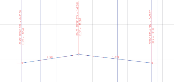
Figure 10.8 A completed cul-de-sac profile
You now have a proposed profile that is acceptable to use in the cul-de-sac baseline. Check your work against 1002_EOPProfile_FINISHED.dwg or 1002_EOPProfile_METRIC_FINISHED.dwg to see how your stations and elevations compare. You do not need to save the drawing file.
Putting the Pieces Together
You have all the pieces in place to perform the first iterations of this cul-de-sac design.
The following exercise will walk you through the steps to put the cul-de-sac together. You will complete several steps and let the corridor build to observe what is happening at each stage. This exercise will also encourage you to get comfortable using the Corridor Properties dialog to make design modifications.
- Open the
1003_Cul-de-SacDesign.dwg(1003_Cul-de-SacDesign_METRIC.dwg) file, which you can download from this book's web page. - This drawing contains the cul-de-sac centerline alignment and profile, the EOP alignment and profile, and the assemblies needed to complete the process.
- Click the corridor.
 From the contextual tab Modify Corridor panel, click Add Baseline.
- In the Create Corridor Baseline dialog, select ROAD E CUL-DE-SAC from the drop-down list. Click OK to continue.
- In the Select a Profile dialog, select FG-ROAD E CUL-DE-SAC from the drop-down list. Click OK to continue.
 From the contextual tab Modify Region panel, select Add Regions.
- At the
Select a baseline:prompt, click over the cul-de-sac alignment in the drawing. - At the
Specify the region start station:prompt, type 0 ↵ Alternatively, you could snap to the end of the corridor at this location. - At the
Specify the region end station:prompt, type 369.17 (113.26 for metric) ↵. Alternatively, you could snap to the edge of the corridor at this location. - In the Create Corridor Region dialog, under Assembly, select Curb Returns from the drop-down list. Click OK to continue.
- In the Target Mapping dialog, in the Object Name column, click <None> next to Target Surface and select Existing Surface from the drop-down list in the Pick A Surface dialog. Click OK to dismiss the Pick A Surface dialog, and click OK again to dismiss the Target Mapping dialog.
- Press the Esc button on your keyboard to end the command.
The curb return assembly has been wrapped around the cul-de-sac, as shown in Figure 10.9. However, the curve frequency needs to be increased to mimic the curvature of the cul-de-sac bulb. Also, an offset and elevation target will have to be set so that the pavement of the assembly stretches to connect horizontally and vertically to the centerline design of ROAD E.
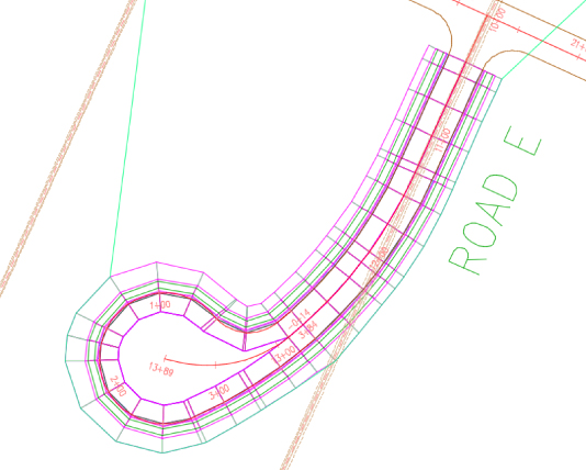
Figure 10.9 Cul-de-sac region before configuring frequency and targets
 On the contextual tab, Modify Region panel, select Edit Frequency.
- At the
Select a region to edit:prompt, click anywhere inside the cul-de-sac portion of the corridor. Be careful not to select inside the “donut hole” in the center of the cul-de-sac. - In the Frequency To Apply Assemblies dialog, change the Curve Increment value to 5 (1.5 for metric). Click OK to dismiss the dialog.
- Press the Esc key to end the command.
- To stretch the pavement to meet the horizontal and vertical centerline of ROAD E, on the contextual tab Modify Region panel, select Edit Targets.
- At the
Select a region to edit:prompt, click anywhere inside the cul-de-sac portion of the corridor. Be careful not to select inside the “donut hole” in the center of the cul-de-sac. - In the Target Mapping dialog in the Width or Offset Targets section, click in the Object Name column next to Width Alignment. Note the name of the subassembly in the Subassembly column.
- In the Set Width Or Offset Target dialog, under Select Alignments, click ROAD E.
- Click the Add button to place it on the list below.
- Click OK to continue.
- Back in the Target Mapping dialog in the Slope or Elevation Targets section, click in the Object Name column next to Outside Elevation Profile. Note the name of the subassembly in the Subassembly column.
- In the Set Slope Or Elevation Target dialog, select ROAD E as the alignment.
- Under Select Profiles, choose FG-ROAD E and click the Add button to place it on the list below. You may need to change the width of the Name column to see the full profile name.
- Click OK to dismiss the dialog.
- Click OK again to close the Target Mapping dialog.
- The corridor is completely modeled (see Figure 10.10).
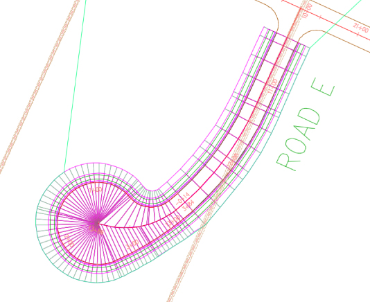
Figure 10.10 The completed cul-de-sac corridor
- With the corridor still selected, open Corridor Properties from the contextual tab.
- On the Parameters tab, inspect the baselines and regions that are accumulating in your corridor, as shown in Figure 10.11.
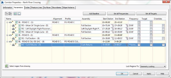
Figure 10.11 Multiple baselines and regions in Corridor Properties
The files 1003_Cul-de-SacDesign_FINISHED.dwg and 1003_Cul-de-SacDesign_METRIC_FINISHED.dwg are available for you to check your work.
Troubleshooting Your Cul-de-Sac
People make several common mistakes when modeling their first few cul-de-sacs:
- Your cul-de-sac appears with a large gap in the center. If your curb line seems to be modeling correctly but your lanes are leaving a large empty area in the middle (see Figure 10.12), chances are pretty good that you forgot to assign targets or perhaps assigned the incorrect targets.
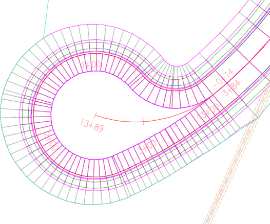
Figure 10.12 A cul-de-sac without targets
You can fix this problem by opening the Target Mapping dialog for your region and checking to make sure you assigned the road centerline alignment and FG profile for your targets. Also, check to see if you assigned these targets to the wrong subassembly.
To pinpoint the location of errors, use the Edit Targets tool from the Modify Region panel of the Corridor contextual ribbon. Edit targets one region at a time to avoid confusion.
- Your cul-de-sac appears to be backward. Occasionally, you may find that your lanes wind up on the wrong side of the EOP alignment, as shown in Figure 10.13. The direction of your alignment will dictate whether the lane should be on the left or right side. In the example from the previous exercise, the alignment was running counterclockwise around the cul-de-sac bulb; therefore, the lane was on the left side of the assembly.
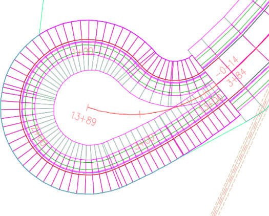
Figure 10.13 A cul-de-sac with the lanes modeled on the wrong side without targets
You can fix this problem by changing the assembly applied to the region to one that was created for the correct side or reversing the alignment.
- Your cul-de-sac drops down to 0. A common problem when you first begin modeling cul-de-sacs, intersections, and other corridor components is that one end of your baseline drops down to 0. You probably won't notice the problem in plan view, but once you build your surface or rotate your corridor in 3D (see Figure 10.14), you'll see it. This problem will always occur if your region station range extends beyond the proposed profile.

Figure 10.14 A corridor viewed in 3D showing a drop down to 0 (bottom)
- To fix this problem, make sure your region station range corresponds with the design profile length. You may need to extend the design profile in some cases, but usually restricting the station range of the region will do the trick.
- Your cul-de-sac seems flat. When you're first learning the concept of targets, it's easy to mix up baseline alignments and target alignments. In the beginning, you may accidentally choose your EOP alignment as a target instead of the road centerline. If this happens, your cul-de-sac will look similar to Figure 10.15.
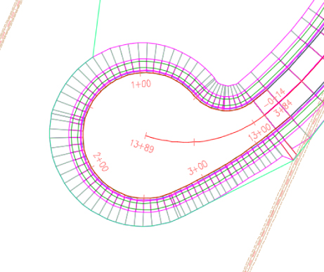
Figure 10.15 A flat cul-de-sac with the wrong lane target set
- You can fix this problem by opening the Target Mapping dialog for this region and making sure the target alignment is set to the road centerline and the target profile is set to the road centerline FG profile.
Moving Up to Intersections
Now that you have a thorough understanding of cul-de-sacs, you're ready to take on intersections.
The steps that follow apply to all intersections, regardless of whether it is a T-shaped intersection, a four-way intersection, perfectly perpendicular, or skewed at an angle.
![]() When you build your corridor model, chances are that it will not be graded perfectly, and you may need to tweak it to perfect it. This is why you build the model in the first place, so you can easily see if and where the model fails. Design flaws are difficult to catch right away when you're dealing with a two-dimensional model.
When you build your corridor model, chances are that it will not be graded perfectly, and you may need to tweak it to perfect it. This is why you build the model in the first place, so you can easily see if and where the model fails. Design flaws are difficult to catch right away when you're dealing with a two-dimensional model.
Plan what alignments, profiles, and assemblies you'll need to create the right combination of baselines, regions, and targets to model an intersection that will interact the way you want. It helps to create a simple sketch, as shown in Figure 10.16.
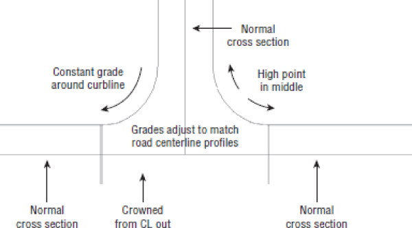
Figure 10.16 Plan your intersection model in sketch form.
Figure 10.17 shows a sketch of required baselines. As you saw in the previous example, baselines are the horizontal and vertical foundations of a corridor. Each baseline consists of an alignment and its corresponding finished ground (FG) profile. You may never have thought of edge of pavement in terms of profiles, but after you build a few intersections, thinking that way will become second nature. The Intersection tool on the Create Design panel of the Home tab will create EOP baselines as curb return alignments for you, but it will rely on your input for curb return radii.
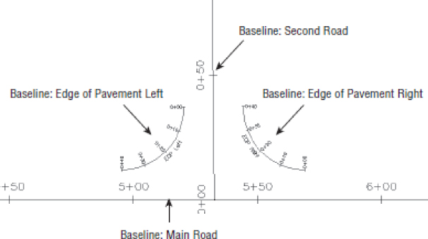
Figure 10.17 Required baselines for modeling a typical intersection
Figure 10.18 breaks each baseline into regions where a different assembly or different target will be applied. Once the intersection has been created, target mapping as well as other particulars can be modified as needed.
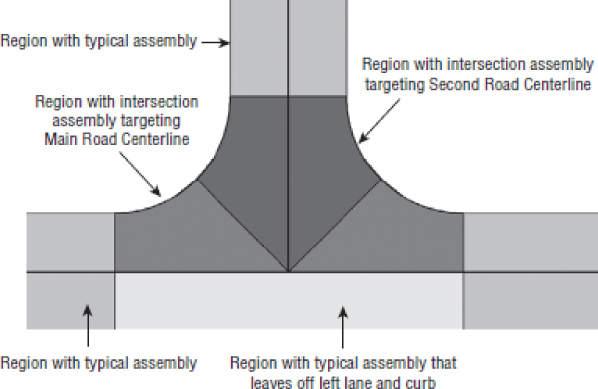
Figure 10.18 Required regions for modeling an intersection created by the Intersection tool
Using the Intersection Wizard
![]() All the work of setting baselines, creating regions, setting targets, and applying the correct frequencies can be done manually for an intersection. However, Autodesk® AutoCAD® Civil 3D® software contains an automated Intersection tool that can handle many types of intersections.
All the work of setting baselines, creating regions, setting targets, and applying the correct frequencies can be done manually for an intersection. However, Autodesk® AutoCAD® Civil 3D® software contains an automated Intersection tool that can handle many types of intersections.
On the basis of the schematic you drew of your intersection, your main road will need several assemblies to reflect the different road cross sections. Figure 10.19 shows the full range of potential assemblies you may need in an intersection and the design situations in which they may arise.
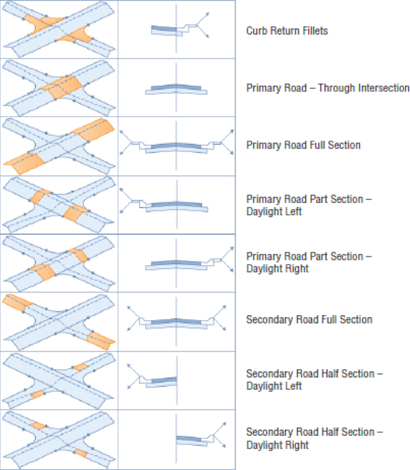
Figure 10.19 Various assembly schematics and applications
This exercise will take you through building a typical intersection with a couple of right-turn lanes using the Create Intersection Wizard:
- Open the
1004_Intersection.dwg(1004_Intersection_METRIC.dwg) file, which you can download from this book's web page.You'll start by building a four-way intersection for ROAD A and ROAD D.
- From the Home tab Create Design panel, choose the Intersections Create Intersection tool.
- At the
Select intersection point:prompt, choose the intersection of the two existing alignments. (Hint: The Intersection Osnap will automatically turn on and be active.) - At the
Select main road alignment <or press enter key to select from list>:prompt, click the ROAD A alignment that runs from west to east.The Create Intersection – General dialog will appear (Figure 10.20).
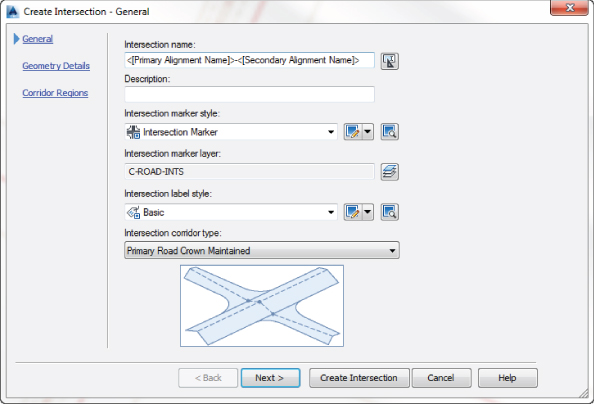
Figure 10.20 The General page of the Create Intersection Wizard
- Set Intersection Corridor Type to All Crowns Maintained and click Next.
- In the Geometry Details page (Figure 10.21), verify that ROAD A is the primary road by looking at the Priority list. If ROAD A is not at the top of the list, use the arrow buttons on the right side to reorder the roads.
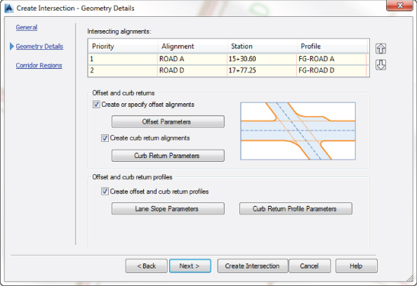
Figure 10.21 The Geometry Details page of the Create Intersection Wizard
- Click the Offset Parameters button, and do the following in the Intersection Offset Parameters dialog:
- Set the offset values for both the left and right sides to 14′ (4.5 m) for both ROAD A and ROAD D.
- Fill in the check box for Create New Offsets From Start To End Of Centerlines. This will ensure that the turn lanes you're about to create will have targets to meet.
At this step, the screen should resemble Figure 10.22.
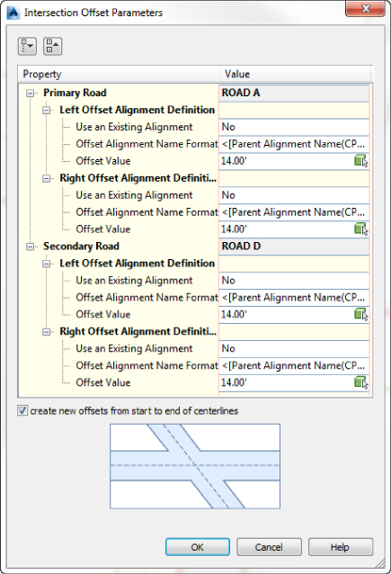
Figure 10.22 Intersection Offset Parameters dialog
- Click OK to close the Intersection Offset Parameters dialog.
- On the Geometry Details page, click the Curb Return Parameters button to enter the Intersection Curb Return Parameters dialog.
- For the NE and SW quadrants, place a check mark next to Widen Turn Lane For Incoming Road.
You will be creating right-turn lanes for ROAD A. Notice how the dialog changes when the check box is filled to show widening parameters.
- Click the Next button at the top of the dialog to move from quadrant to quadrant.
You will see a schematic name of the quadrant listed at the top of the dialog that corresponds to the glyph. As shown in Figure 10.23, the temporary glyph will help you determine which quadrant you are currently modifying.
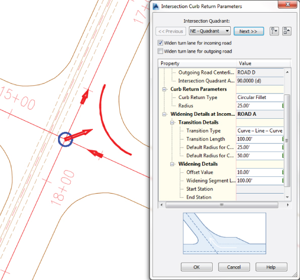
Figure 10.23 Adding lane widening to the NE – Quadrant of the intersection
When you reach the last quadrant, you will see that the Next button is grayed out. This means that you have successfully worked through all four curb returns.
- Click OK to return to the wizard's Geometry Details page.
Some locales require that lane slopes flatten out to a 1 percent cross-slope in an intersection. If this is the case for you, you can change the lane slope parameters in the Intersection Lane Slope Parameters dialog (Figure 10.24). In this exercise you will leave this setting at -2%.
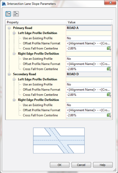
Figure 10.24 Lane slope parameters control the cross-slope in the intersection.
Civil 3D performs the task of generating the curb return profile. The profile will be at least as long as the rounded curb plus the turn lanes that are added in this exercise. If you wish to have Civil 3D generate even more than the length needed, you can specify that in the Intersection Curb Return Profile Parameters dialog (Figure 10.25). This dialog is actually a series of dialogs based on quadrant, as was the Curb Return Parameters dialog. According to Figure 10.25, the alignment and profile for the SE - Quadrant curb return will be extended 25′ beyond its PCs and PTs. And how is this useful? You'll find out in the upcoming section called “Manual Intersections.”
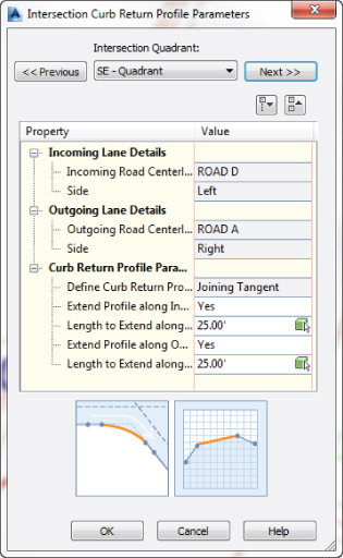
Figure 10.25 Intersection Curb Return Profile Parameters options extend the Civil 3D–generated profile beyond the curb returns by the value specified.
You will be keeping all default settings in both the Lane Slope Parameters area (Figure 10.24) and the Curb Return Profile Parameters area (Figure 10.25).
- For the NE and SW quadrants, place a check mark next to Widen Turn Lane For Incoming Road.
- Click Next to continue to the Corridor Regions page of the Create Intersection Wizard (Figure 10.26).
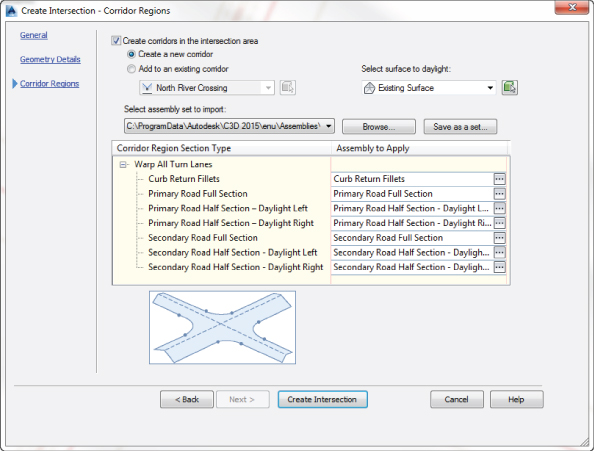
Figure 10.26 The Corridor Regions page of the Create Intersection Wizard drives the assemblies used in the intersection.
The Corridor Regions page is where you control which assemblies are used for the different design locations around the intersection. Clicking each entry in the Corridor Region Section Type list will give you a preview of what each assembly type should look like and where in the intersection it's applied (as shown at the bottom of Figure 10.26). If your assemblies have the same names as the default assemblies, they will be pulled from the current drawing. Alternatively, you can click the ellipsis to select any assembly from the drawing, which is what you will be doing in this example.
If you didn't have all the necessary assemblies created in your drawing at this point, you could still create your intersection with the default assemblies. You could always modify the default assemblies with your own criteria and subassemblies after they are brought in.
- On the Corridor Regions page, do the following:
- Click Add To An Existing Corridor to place the intersection in the North River Crossing corridor.
- Verify that Select Surface To Daylight is set to Existing Surface.
- In the Corridor Region Section Type list, set the following:
Corridor Region Section Type Assembly To Apply Curb Return Fillets Curb Returns Primary Road Full Section Full Section Primary Road Half Section - Daylight Left Left Half Primary Road Half Section - Daylight Right Right Half Secondary Road Full Section Full Section Secondary Road Half Section - Daylight Left Left Half Secondary Road Half Section - Daylight Right Right Half - Giving each assembly a friendly, meaningful name will keep things less confusing.
- Click Create Intersection.
After a few moments of processing, you will see a corridor appear at the intersection of the roads. Use the
REGENcommand if you do not see the frequency lines. Your corridor should now resemble Figure 10.27.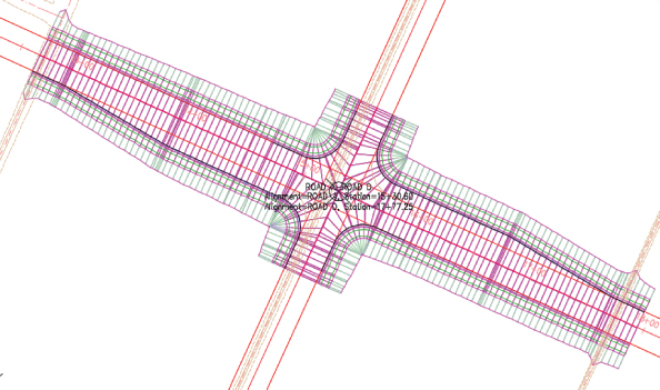
Figure 10.27 The completed intersection
- Select the corridor, and from the Corridor contextual tab Modify Corridor panel, select Corridor Properties.
- Switch to the Parameters tab of the Corridor Properties dialog and highlight one of the regions toward the bottom in the list, as shown in Figure 10.28.
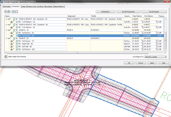
Figure 10.28 One way to modify regions is to use the Parameters tab in Corridor Properties. The selected region will highlight graphically.
Notice how the region highlighted in the Parameters tab is outlined in the graphic. This will help you determine which region to edit.
 To move from region to region without searching through the overwhelming list of baselines and regions, use the Select Region From Drawing button.
 - Click Cancel to close Corridor Properties and press Esc to deselect.
Next you will create a three-way intersection.
- Switch to the Parameters tab of the Corridor Properties dialog and highlight one of the regions toward the bottom in the list, as shown in Figure 10.28.
- In your drawing, pan northward to the intersection of ROAD C and ROAD D.
- From the Home tab Create Design panel, choose the Intersections Create Intersection tool.
- At the
Select intersection point:prompt, choose the intersection of the two existing alignments.You will not be prompted to pick a main/primary road alignment for three-way intersections. The Intersection tool automatically configures the through road as the primary road.
- On the General page of the Intersection wizard, set the Intersection Corridor Type to All Crowns Maintained and click Next.
- On the Geometry Details page, accept the defaults and click Next.
- On the Corridor Regions page, do the following:
- Click Add To An Existing Corridor to place the intersection in the North River Crossing corridor.
- Verify that Select Surface To Daylight is set to Existing Surface.
- In the Corridor Region Section Type list, set the following:
Corridor Region Section Type Assembly to Apply Curb Return Fillets Curb Returns Primary Road Full Section Full Section Primary Road Half Section - Daylight Left Left Half Primary Road Half Section - Daylight Right Right Half Secondary Road Full Section Full Section Secondary Road Half Section - Daylight Left Left Half Secondary Road Half Section - Daylight Right Right Half - Before creating this intersection, click the Save As A Set button so this configuration of assemblies can be reused on the other two three-way intersections.
- Name your file
NorthRiverand click Save to continue.
- Click the Create Intersection button to add this intersection to the North River Crossing corridor.
- Repeat steps 15–19 for the intersection of ROAD C and ROAD B with the following exceptions:
- On the Intersection Offset Parameters dialog, turn off Create New Offsets From Start To End Of Centerlines.
- On the Corridor Regions page, click Browse to choose the assembly set you just created.
- In the Select Assembly Set File dialog, select the
NorthRiver.xmlfile and click Open to import.This may take a few seconds, so wait for it.
- Do not forget to add the intersection to the North River Crossing corridor.
- Create the intersection.
- Repeat steps 15–19 for the intersection of ROAD A and ROAD E with the following exceptions:
- You will not need to browse for the assembly set. The wizard will remember the last assembly set used.
- Do not forget to add the intersection to the North River Crossing corridor.
- Create the intersection.
You should have four intersections in addition to your cul-de-sac modeled in your drawing, as shown in Figure 10.29.
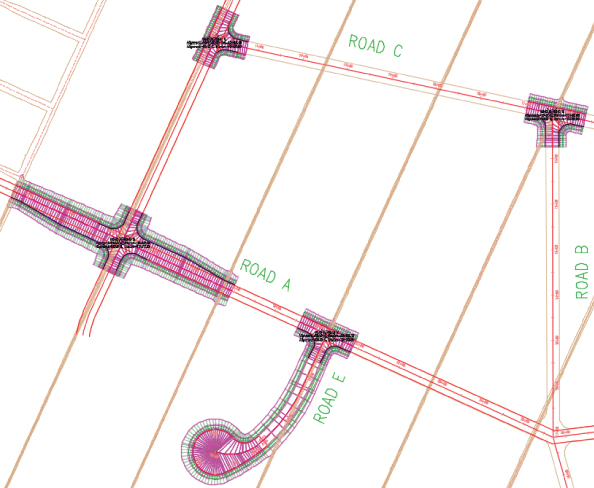
Figure 10.29 Four intersections and a cul-de-sac, all modeled in the North River Crossing corridor
- Save and close the drawing when you have completed the exercise.
The files
1004_Intersection_FINISHED.dwgand1004_Intersection_METRIC_FINISHED.dwgare available for your review.
Creating Intersections Manually
You will begin this section by visiting an intersection with unusual circumstances that must be built manually. Then we will discuss other issues you can experience with intersections.
- Open the
1004_Intersection_FINISHED.dwg(1004_Intersection_METRIC_FINISHED.dwg) file, which you can download from this book's web page. - Zoom into the intersections of the ROAD A and ROAD B alignments.
- From the Home tab, on the Create Design panel Intersections tool, select Create Intersection and pick the intersection of ROAD A and ROAD B.
- At the
Select main road alignment <or press enter key to select from list>:prompt, click the ROAD A alignment that runs from west to east. - On the General page of the Create Intersection Wizard, for Intersection Corridor Type select All Crowns Maintained. Then click Next.
- On the Geometry Details page, you'll be using the defaults for all parameters, so click Next.
- On the Corridor Regions page, do the following:
- Turn on Add To Existing Corridor.
- Set the assemblies to the following:
Corridor Region Section Type Assembly to Apply Curb Return Fillets Curb Returns Primary Road Full Section Full Section Primary Road Half Section - Daylight Left Left Half Primary Road Half Section - Daylight Right Right Half Secondary Road Full Section Full Section Secondary Road Half Section - Daylight Left Left Half Secondary Road Half Section - Daylight Right Right Half - Click Create Intersection.
The intersection will be created. Event Viewer will open displaying a number of errors, as shown in Figure 10.30.
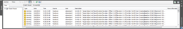
Figure 10.30 Errors resulting from creating final intersection
Upon looking through the errors in Event Viewer, you'll discover that they are all the same error occurring at different stations. Each mentions a target object not being found. The subassembly involved is LaneSuperelevationAOR and the Target name is Outside Elevation. Since the Intersection tool uses profiles for elevation targets, there must be a problem with one of the profiles that the tool created. A quick way to figure out which one(s) would be to examine the intersection in 3D.
- On the ribbon, make the View tab current and do the following:
- On the Model Viewports panel Viewport Configuration tool, select Two: Vertical to split your drawing window into two viewports.
- Click in the right viewport to make it current.
- On the Views panel Named View list, make the 3D named view current.
Your viewport configuration should be similar to Figure 10.31.
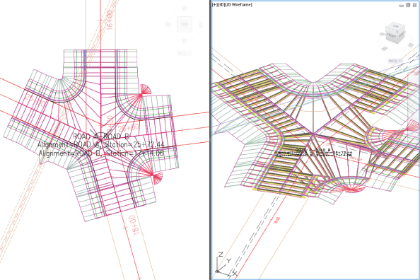
Figure 10.31 A combination of viewport configurations can help you keep an eye on your corridor design.
For some reason, you have two quadrants in this intersection that decided to set down at elevation zero. You could spend a lot of time trying to seek out the reasons for this, but if you're like most of us, you're in a time crunch and would like to finish up this roadway model. Before we delve into creating manual intersections, it's important that you look at a couple of things before moving on.
If you look at the profile properties for both the NE and SE quadrants on the Prospector under Alignments
Curb Returns, you'll see that the profile is empty of station and elevation data (Figure 10.32), so this is one area where the Intersection tool failed. However, according to the errors, the targeting problems are occurring along the ROAD B baseline, so what is happening there?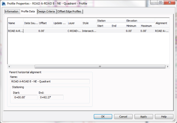
Figure 10.32 Curb return profile is empty of station and elevation data.
If you open up Corridor Properties, scroll all the way down to the bottom of the list on the Parameters tab, select one of the regions, click the Target ellipsis, and open the Set Slope Or Elevation Target dialog for the left lane, you'll see that the “bad” profiles show up for targeting there as well.
Even if you made manual overrides to cause your corridor to use relevant data, you will still receive errors in Event Viewer because the Intersection tool does not want to let go of the profiles and settings it created. The upside to this behavior is that autogenerated intersections will always update. The downside to this behavior is when you are in situations like this where the tool failed in an area and you need to make manual adjustments. The best thing to do here is to “turn the intersection off.” The Intersection tool did do a lot of the heavy lifting for you, so all is not lost.
- On the Model Viewports panel
- Press the Esc key a few times to make sure nothing is currently selected. This is always a good thing to do when you are about to press the Delete key.
- In the left viewport, click the intersection marker (X with a circle imposed at the center). When you do so, the Intersection contextual ribbon will appear.
Examine the contextual ribbon. Notice the tools for editing offset, curb return, lane slopes, and curb return parameters. If any of the parameters set in the Intersection wizard need to change, these tools can be used to reconfigure the intersection.
- Press the Delete key.
The contextual ribbon closes, the intersection marker and label disappear, and the entry for this intersection on Prospector will no longer be found.
The next step is to re-create the two curb return profiles with relevant station and elevation data.
- In Prospector, in Alignments Curb Return Alignments, right-click ROAD A-ROAD B - NE Quadrant and choose Select.
- Select Surface Profile from the Launch Pad panel on the contextual ribbon.
- In the Create Profile From Surface dialog, do the following:
- Under Select Surfaces, select North River Crossing Surface - Top.
- Click the Add button to add it to the profile list.
- Click Draw In Profile View.
- In the Create Profile View dialog, click Create Profile View and place the profile in an open area in your drawing.
If you take a look at the profile, the surface that is being displayed in profile is doing exactly what your corridor is doing: taking a dive down to elevation 0 where the quadrant begins and ends. Here is where you get to fill in the gap again.
- On the Home tab Create Design Panel, select Profile and open the Profile Creation Tools.
- At the
Select profile view to create profile:prompt, select the profile view for the curb return. - In the Create Profile dialog, change the text in the Name field to FG-<[Alignment Name]>. Click OK to continue.
- On the Profile Layout Tools toolbar, select Draw Tangents, and using your Endpoint Osnap, bridge the gap as shown in Figure 10.33.
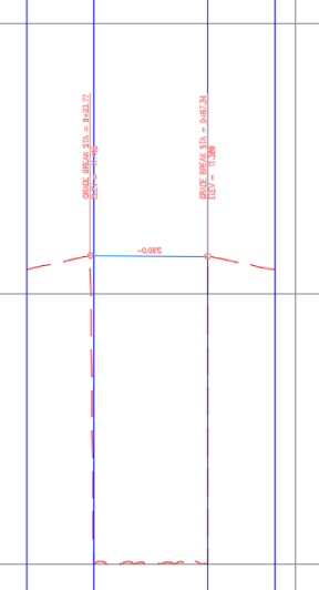
Figure 10.33 Filling in the elevation gap in profile view
- Press ↵ to end the command. Close the Profile Layout Tools toolbar.
You have created an actual profile that can be used in the NE quadrant of this intersection. Next, you'll address the SE quadrant.
- Repeat steps 12–20 for the curb return alignment called ROAD A-ROAD B - SE Quadrant.
- Using the left viewport, pan back over to the troubled intersection.
- Select the corridor to reveal the contextual ribbon.
- On the contextual ribbon, select Corridor Properties and do the following:
-
 On the Parameters tab, locate BL - ROAD A-ROAD B - NE - Quadrant (the name of the baseline may have a counter behind it depending how many times the Intersection command was executed). It may be helpful to simplify the list using the Collapse All Categories button in the top left of the dialog. You may use the Select Region From Drawing button as an alternative to searching the list.
- In the Profile column, click the profile name for that baseline to change the selection.
- In the Select A Profile dialog, change the selection to FG-ROAD A-ROAD B - NE - Quadrant. Click OK to continue.
- Next, locate BL - ROAD A-ROAD B - SE - Quadrant.
- In the Profile column, click the profile name for that baseline to change the selection.
- In the Select A Profile dialog, change the selection to FG-ROAD A-ROAD B - SE - Quadrant. Click OK to continue.
- Click OK in the Corridor Properties and rebuild the corridor if prompted.
Event Viewer will pop up.
- In Event Viewer, clear all the events being reported using the Action button.
Although the right viewport is now showing a good-looking intersection, you'll want to take the following steps to ensure that Event Viewer isn't picking up any more problems with the corridor.
- On the contextual ribbon, on the Modify Regions tab, select Edit Targets.
- At the
Select a region to edit:prompt, select the RG - Full Section region along ROAD B north of the intersection, as indicated by Figure 10.34.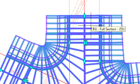
Figure 10.34 Selecting the RG - Full Section region along ROAD B north of the intersection.
- In the Target Mapping dialog, under Slope Or Elevation Targets Outside Elevation Profile for the Left assembly group, click in the Object Name column.
- In the Set Slope Or Elevation Target dialog, do the following:
- In the Selected Entities To Target section, select both profiles on the list.
 Click the Delete Selected Item button to remove both profile targets from the list.
Neither of these targets are needed since you are not widening the road in this area.
- Click OK to close.
- Click OK to close the Target Mapping dialog.
The
Select a region to edit:prompt should still be active. - Select the RG - Left Half region in the north part of the intersection along ROAD B, as indicated by Figure 10.35.
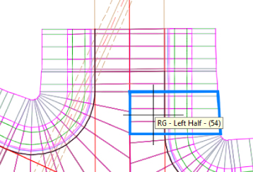
Figure 10.35 Selecting the RG - Left Half region along ROAD B north of the intersection
- Repeat steps 28–30. Just be aware that sometimes the Intersection tool will throw in the alignment as an elevation target instead of the bad profile. If you find that to be the case, remove the alignment from the list.
The
Select a region to edit:prompt should still be active. - Select the RG - Full Section region in the south part of the intersection along ROAD B, as indicated by Figure 10.36.
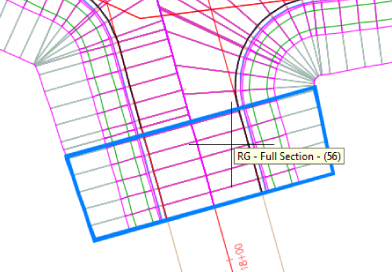
Figure 10.36 Selecting the RG - Full Section region along ROAD B south of the intersection
- Repeat steps 28–30.
- Press ↵ to end the command.
Now if you were to clear the events out of Event Viewer and rebuild the corridor, you would receive no errors. It's better to reserve the error list for those items that you need to address.
The files 1005_ManualIntersection_FINISHED.dwg and 1005_ManualIntersection_METRIC_FINISHED.dwg are available for your review.
Troubleshooting Your Intersection
The best way to learn how to build advanced corridor components is to go ahead and build them, make mistakes, and try again. This section provides some guidelines on how to “read” your intersection to identify what steps you may have missed.
- Your lanes appear to be backward. Occasionally, you may find that your lanes wind up on the wrong side of the EOP alignment, as in Figure 10.37. The most common cause is that your assembly is backward from what is needed based on your alignment direction.
Figure 10.37 An intersection with the lanes modeled on the wrong side
Fix this problem by editing your subassembly to swap the lane to the other side of the assembly. If the assembly is used in another region that is correct, just make a new assembly that is the mirror image of the other assembly and apply the new one to the alignment.
Since so many design elements rely on the alignment as their base, it is better to add a new assembly rather than reversing the direction of the alignment.
- Your intersection drops down to zero A common problem when modeling corridors is the cliff effect, where a portion of your corridor drops down to zero. You probably won't notice in plan view, but if you rotate your corridor in 3D using Object Viewer (see Figure 10.38), you'll see the problem. The most common cause for this phenomenon is incorrect region stationing.
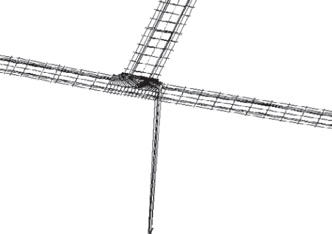
Figure 10.38 A corridor viewed in 3D, showing a drop down to zero
Fix this problem by making sure your baseline profile exists where you need it, and make note of the station range. Set your station range in the corridor to be within the correct range.
- Your lanes extend too far in some directions. There are several variations on this problem, but they all appear similar to Figure 10.39. All or some of your lanes extend too far down a target alignment, or they may cross one another, and so on.
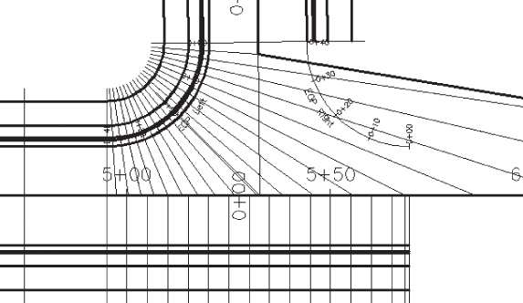
Figure 10.39 The intersection lanes extend too far down the main road alignment.
- This occurs when a target alignment and profile have been omitted for one or more regions. In the case of Figure 10.39, the EOP Left baseline region was set to only one alignment. In an intersection, you need two targets in a corner region to model the road correctly. You would see a similar issue appear if the Selection Choice If Multiple Targets Are Found option were set to Target Farthest From Offset.
- Your lanes don't extend far enough. If your intersection or portions of your intersection look like Figure 10.40, you neglected to set the correct target alignment and profile.
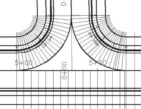
Figure 10.40 Intersection lanes don't extend out far enough.
- You can fix this problem by opening the Target Mapping dialog for the appropriate regions and double-checking that you assigned targets to the right subassembly. It's also common to accidentally set the target for the wrong subassembly if you use Map All Targets or if you have poor naming conventions for your subassemblies.
Finishing Off Your Corridor
Now it's time for you to fill in another kind of gap in the corridor. You will be filling in the corridor between the intersections you created.
- Open the
1005_ManualIntersection_FINISHED.dwg(1005_ManualIntersection_METRIC_FINISHED.dwg) file, which you can download from this book's web page. - On Prospector, expand the Intersections branch.
- Zoom into the ROAD A-ROAD E intersection and select it to reveal its grips.
- Grab the leftmost diamond shape region grip, which coincides with ROAD A alignment, and drag it over to the adjacent diamond shape region grip in the ROAD A-ROAD E intersection, as shown in Figure 10.41.

Figure 10.41 Stretching the region to match up with adjacent region.
- Notice how your intersections become out of date according to the yellow alert shield that appears next to each.
- Right-click ROAD A-ROAD E and select Update Regions And Rebuild Corridor.
- When the Intersections - Update Corridor Regions dialog opens, select Continue With Update.
- Notice how the stretched region returns to its original position.
- This could be a problem if you are relying on the dynamic dependencies of your intersections to keep your corridor updated. Next, you'll try an alternative method of filling in the gaps.
- Select the corridor, and on the contextual ribbon select Add Baseline from the Modify Corridor panel and do the following:
- In the Create Corridor Baseline dialog, choose ROAD A as the Horizontal Alignment. Alternatively, you can use the green select object button in the dialog. Click OK to continue.
- In the Select A Profile dialog, select FG-ROAD A. Click OK to continue.
- On the contextual ribbon, select Add Regions from the Modify Regions panel, and do the following:
- At the
Select a baseline:prompt, place your cursor over the ROAD A alignment and left-click.The Select A Baseline dialog opens. The command ascertains that there are four baselines associated with ROAD A. The first three on the list belong to the three intersections on ROAD A.
- Select the last baseline on the list and click OK.
- At the
Specify region start station prompt, snap to the diamond grip, as shown in Figure 10.42.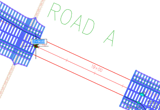
Figure 10.42 Defining the region start station
When selecting the region start station, it must be an earlier station than the region end station that you will select next.
- At the
Specify region end station prompt, snap to the diamond grip, as shown in Figure 10.43.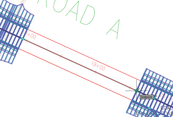
Figure 10.43 Defining the region end station
- In the Create Corridor Region dialog, select the Full Section assembly and click OK to apply.
- In the Target Mapping dialog, in the Object Name column next to Surfaces, click <Click Here To Set All> and then select Existing Surface.
- Click OK to continue.
- Click OK to close the Target Mapping dialog.
Your new baseline-region should resemble Figure 10.44.
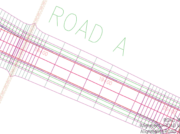
Figure 10.44 Filling in the gap with a new baseline region
The Add Region command is still active.
- Repeat steps 9c–9h for the rest of the empty regions along ROAD A.
- When the regions along ROAD A are complete, press ↵ to end the Add Regions command.
- At the
Optionally, you may repeat steps 8–9 to fill in the gaps in this corridor along the remaining areas of ROADs B, C, and D.
The files 1006_FillingCorridorGaps_FINISHED.dwg and 1006_FillingCorrodorGaps_METRIC_FINISHED.dwg are available for your review.
Using an Assembly Offset
In Chapter 9, you completed a road-widening example with a simple lane transition. Earlier in this chapter, you worked with intersections and cul-de-sacs. These are just a few of the techniques for adjusting your corridor to accommodate a widening, narrowing, interchange, or similar circumstances. There is no single method for building a corridor model; every method discussed so far can be combined in a variety of ways to build a model that reflects your design intent.
Another tool in your corridor-building arsenal is the assembly offset. In Chapter 8, “Assemblies and Subassemblies,” you had your first glimpse of an offset assembly, but in the example that follows you will have a chance to use one for a bike path design.
Notice in Figure 10.45 how the frequency lines in the corridor are running perpendicular to the main alignment. The bike path is an alignment that is not a constant offset through the length of the corridor. In this scenario, the cross section of the bike path itself is skewed. This could prove problematic when computing end area volumes for the bike path pavement. This is the result of using an assembly where all of the design is based on one main baseline assembly.
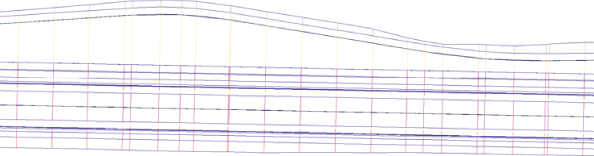
Figure 10.45 A bike path modeled with a traditional assembly
There are several advantages to using an offset assembly instead of creating an additional, separate assembly. The offset assembly requires its own alignment and profile for design. In the corridor that results, a secondary set of frequency lines is generated perpendicular to the offset alignment, as shown in Figure 10.46. Additionally, you can use a marked point assembly to model the ditch between the bike path and the main road.
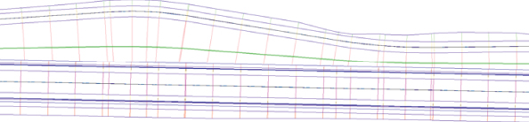
Figure 10.46 Modeling a bike path with an assembly offset
There are many uses of offset assemblies besides bike paths. Typical examples of when you'll use an assembly offset include transitioning ditches, divided highways, and interchanges. The assembly in Figure 10.47, for example, includes two assembly offsets.
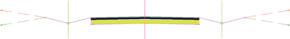
Figure 10.47 An assembly with two offsets representing roadside swale centerlines
When you use an assembly with an offset in your corridor, you must assign an alignment and profile to it. The only restriction to the offset assembly is that it can't use the same alignment or profile as the main part of the assembly. In the case where you want your offsets to follow the same elevation, you will need to use the Superimposed Profile tool to effectively make a copy of the desired profile.
In this exercise, you will model a bike path with an assembly offset:
- Open the
1007_BikePath.dwg(1007_BikePath_METRIC.dwg) file, which you can download from this book's web page. - Locate the assembly in the Prospector tab, right-click, and click Zoom To.
You'll see an incomplete assembly called Road With GR And Bikepath.
 Click the main assembly marker, and then from the Assembly contextual tab Modify Assembly panel, click Add Offset.
- At the
Specify offset location:prompt, click to the left of the Road With GR And Bikepath assembly, leaving enough room for the bike lane and ditch.Your result should look like Figure 10.48. The warning symbols indicate that you can no longer use the assembly for roads where superelevation occurs at points other than the centerline. Superelevation at the crown will still work, which is the situation used here.
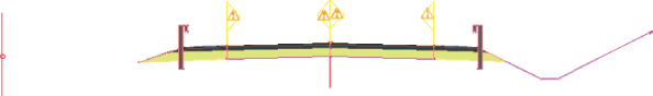
Figure 10.48 Road With GR And Bikepath assembly, so far
- Press Ctrl+3 to open the subassembly tool palette.
- Switch to the Basic tab, and select the BasicLane subassembly.
- In the Advanced parameters in the Properties palette, set Side to Right and Width to 5′ (1 m).
- Click to place the subassembly on the offset assembly, and click the offset assembly again to form the left side.
Your assembly should now look like Figure 10.49.
Figure 10.49 Road With GR And Bikepath assembly with the BasicLane subassembly as a bike path
Next, you will use a MarkPoint assembly to set the stage for building a ditch between the bike path and the main road.
- Switch to the Generic tab in the subassembly tool palette, and click the MarkPoint subassembly.
- Change Point Name on the Properties palette to BIKE (use all capital letters).
- Click the outermost point of the left shoulder subassembly.
Your marker will look like Figure 10.50. Note that the point code defaults to MarkedPoint in the subassembly parameters but can be renamed as needed.
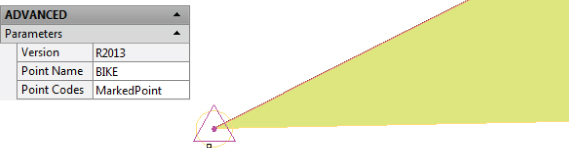
Figure 10.50 A closeup of the MarkPoint subassembly
- From the Generic tab of the subassembly tool palette, click the LinkSlopesBetweenPoints subassembly, and do the following:
- Set Marked Point Name to BIKE (again, use all capital letters).
- Set Ditch Width to 0.5’ (0.15 m).
- Click the right side of the bike path.
The offset assembly will now look like Figure 10.51.
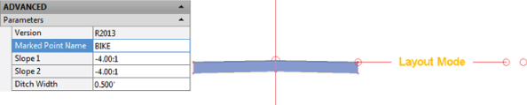
Figure 10.51 The LinkSlopes: BetweenPoints subassembly in layout mode
- Add a LinkSlopeToSurface generic link subassembly, and do the following:
-
- Set Side to Left and Slope to 25%.
- Place the subassembly on the left side of the bike path. Press Esc to finish adding subassemblies and save the drawing.
The completed assembly will look like Figure 10.52.
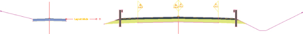
Figure 10.52 The completed assembly with offset
Next, you will create a corridor using this new assembly. You need to have completed the previous exercise before proceeding:
- Continue working in your drawing from the previous exercise.
- From the Home tab Create Design panel, click Corridor and do the following:
- Name the corridor Bike Path.
- Set Alignment to USH 10.
- Set Profile to USH 10 Roadway CL Prof.
- Set Assembly to Road with GR And Bikepath.
- Set Target Surface to Existing Intersection.
- Verify that there is a check mark next to Set Baseline And Region Parameters.
- Click OK.
In the Baseline And Region Parameters dialog, notice that the Offset – (1) is not associated with an alignment (your numbers may vary).
- Click the Alignment field for Offset – (1), select Bike Path from the drop-down list, and click OK.
- Click the Profile field for Offset – (1) and do the following:
- From the Select An Alignment drop-down list, select Bike Path.
- From the Select A Profile drop-down list, select Bike Path FG, and click OK.
The Bike Path alignment is slightly shorter than the main USH 10 alignment, which would cause the “waterfall” effect explained in Chapter 9.
- To prevent corridor errors, do the following:
- Set the start station for the Offset – (1) region to 0+25.00 (0+010.0 for metric users).
- Set the end station to 40+00 (1+220 for metric users).
- Click OK and rebuild the corridor.
Your completed corridor will resemble the example shown earlier in Figure 10.46.
- Select the corridor by clicking on one of the frequency lines anywhere near the middle of the alignment, and click Section Editor.
You may want to change your annotation scale to 1″ = 1′ (1: 1 for metric users) to get an unobstructed view of your masterpiece.
- Explore the finished design by clicking through the Corridor Editor.
At each station, the offset assembly ties back to the main assembly because of the use of the LinkSlopeBetweenPoints subassembly. Your design in the Section Editor should resemble Figure 10.53.
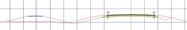
Figure 10.53 Inside the Corridor Section Editor
- On the Section Editor contextual tab Close panel, click Close.
Completed versions of these drawings (
1007_BikePath_FINISHED.dwgand1007_BikePath_METRIC_FINISHED.dwg) are located with the rest of the dataset for your review. - Save and close the drawing.
Understanding Corridor Utilities
You'll now take advantage of some of the corridor utilities found in the Launch Pad panel (Figure 10.54) of the contextual tab.
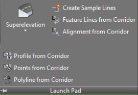
Figure 10.54 A bounty of corridor utilities on the Launch Pad panel
The utilities on this panel are as follows:
- Superelevation This button will jump you to the alignment superelevation parameters. See Chapter 11, “Superelevation,” for a detailed look at how Civil 3D creates banked curves for your design speed.
- Create Sample Lines Corridors and sample lines are both linked to alignments. Civil 3D gives you a shortcut to the sample line creation tool. Chapter 12, “Cross Sections and Mass Haul,” explores the creation and uses of sample lines.
- Feature Lines From Corridor This utility extracts a grading feature line from a corridor feature line. This grading feature line can remain dynamic to the corridor, or it can be a static extraction. Typically, this extracted feature line will be used as a foundation for some feature-line grading or projection grading. If you choose to extract a dynamic feature line, it can't be used as a corridor target due to possible circular references.
- Alignment From Corridor This utility creates an alignment that follows the horizontal path of a corridor feature line. By default, the alignment is categorized as an offset alignment, but it is not tied to the baseline. You can use this alignment to create target alignments, profile views, special labeling, or anything else for which a traditional alignment could be used. Extracted alignments are not dynamic to the corridor. If you place a check box next to the Create Profile option, the resulting profile will be related to the new alignment rather than the baseline.
- Profile From Corridor This utility creates a profile that follows the vertical path of a corridor feature line. This profile appears in Prospector under the baseline alignment and is drawn on any profile view that is associated with that baseline alignment. This profile is typically used to extract edge of pavement (EOP) or swale profiles for a finished profile view sheet or as a target profile for additional corridor design. Extracted profiles are not dynamic to the corridor.
- Points From Corridor This utility creates Civil 3D points that are based on corridor point codes. You select which point codes to use as well as a range of corridor stations. A Civil 3D point is placed at every point-code location in that range. These points are a static extraction and don't update if the corridor is edited. For example, if you extract COGO points from your corridor and then revise your baseline profile and rebuild your corridor, your COGO points won't update to match the new corridor elevations.
- Polyline From Corridor This utility extracts a 3D polyline from a corridor feature line. The extracted 3D polyline isn't dynamic to the corridor. You can use this polyline as is or flatten it to create road linework.
Using Corridor Utilities in Practice
There are many uses for the utilities outlined in this section. Once you get the hang of using some of the corridor utilities, you should find that they are straightforward. In the exercise that follows, you will dabble in the corridor utilities:
- Open the file
1008_CorrUtils.dwg(1008_CorrUtils_METRIC.dwg). - Select the corridor by clicking one of the frequency lines (these are the magenta lines that are perpendicular to the alignment).
- From the Corridor contextual tab Launch Pad panel, click Feature Lines From Corridor.
- At the
Select a Corridor Feature Line:prompt, click the south daylight line (this will be the line that is not a constant offset from the centerline alignment).The Select A Feature Line dialog will appear if you click the daylight line in a cut or fill region. This is because Civil 3D makes two distinct feature lines in these areas. Recall from Chapter 9 that feature lines are formed as a result of marker points with the same name in the assembly connecting together at frequency stations. In other words, why do you have two feature lines here? Because the daylight subassembly creates two marker points at the catch point.
You want the Daylight feature line because it is continuous through the length of the corridor. Daylight_Cut appears only in the cut areas (red) and Daylight_Fill appears only in the fill areas (green). Where the corridor transitions from cut to fill (or fill to cut), you will see a yellow line. Only the Daylight feature line will appear in the transition regions.
- If needed, highlight Daylight and click OK.
- In the Create Feature Line From Corridor dialog (Figure 10.55), clear the check box labeled Create Dynamic Link To The Corridor.
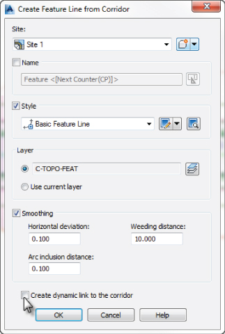
Figure 10.55 Creating a feature line from a corridor without a dynamic link to the corridor
- Leave all other options at their defaults and click OK.
- You should still be in the Create Feature Line From Corridor command and the command line should return to the
Select a Corridor Feature Line:prompt. If you accidentally exited the Feature Lines From Corridor command, start it again from the Launch Pad panel. Click the daylight line on the north side of the road. - Repeat steps 5–7 to create a second feature line out of the north daylight feature line.
- Press Esc to end the command.
- Select the corridor again if it is not already selected.
- From the Corridor contextual tab Launch Pad panel flyout, click Points From Corridor.
- In the Create COGO Points dialog, do the following:
- Toggle on the option For Entire Corridor Range.
- Name the new point group Corridor Stakeout.
- In the Select column, clear all the check boxes except Daylight and ETW, as shown in Figure 10.56. (Hint: Press the Shift key as you click to unselect multiple items at once.)
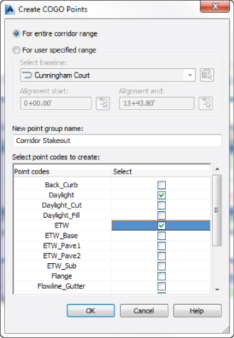
Figure 10.56 Creating points for stakeout along corridor feature lines
- Click OK.
- Save and close the drawing.
Completed versions of this exercise are available with the rest of the dataset.
Using a Feature Line as a Width and Elevation Target
You've gained some hands-on experience using alignments and profiles as targets in an intersection and in a cul-de-sac design. Civil 3D adds options for corridor targets beyond alignments and profiles. You can use grading feature lines, survey figures, or polylines to drive horizontal and/or vertical aspects of your corridor model.
Imagine using an existing polyline that represents a curb for your lane-widening projects without duplicating it as an alignment, or grabbing a survey figure to assist with modeling an existing road for a rehabilitation project. Better yet, what if the object you are targeting is visible to the corridor drawing only as an XRef? The next exercise will lead you through an example where a lot-grading feature line is integrated with a corridor model through an external reference:
- Open the
1009_FeatureLineTarget.dwg(1009_FeatureLineTarget_METRIC.dwg) file, which you can download from this book's web page. Note that the file1009_XREF.dwg(or1009_XREF_METRIC.dwg) must be extracted to the same folder as the main file in order to see it for use in this exercise.This drawing includes a completed assembly and a partially completed corridor. Your task will be to use the feature lines that run through the project as targets in the corridor. These lines are in an external reference file.
- Zoom to the corridor and select it. From the Corridor contextual tab Modify Corridor panel, choose Corridor Properties.
- Switch to the Parameters tab in the Corridor Properties dialog.
- Click the ellipsis button in the Targets field in the RG – Subdivision region. Note that the number following the region will vary. The higher the number, the more previous attempts at building the corridor the authors have made before handing the drawing over to you.
The Target Mapping dialog appears.
- In the Target Mapping dialog, locate the Width Or Offset Targets in the Object Name column. Click the <None> field next to Target Alignment for the Slope-Left subassembly.
The Set Width Or Offset Target dialog appears.
- Choose Feature Lines, Survey Figures And Polylines from the Select Object Type To Target drop-down list (see Figure 10.57).
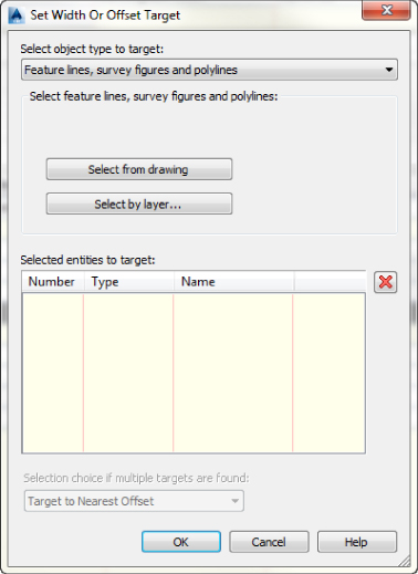
Figure 10.57 The Select Object Type To Target drop-down list at the top of the Set Width Or Offset Target dialog
- In the Set Width Or Offset Target dialog, click the Select From Drawing button. At the
Select feature lines, survey figures or polylines to target:prompt, select the north feature line to the left of the alignment and then press ↵.The Set Width Or Offset Target dialog reappears, with an entry in the Selected Entries To Target area.
- Click OK to return to the Target Mapping dialog.
If you stopped at this point, the horizontal location of the feature line would guide the Slope-Left subassembly, and the vertical information would be driven by the slope set in the subassembly properties. Although this has its applications, most of the time you'll want the feature line elevations to direct the vertical information. The next few steps will teach you how to dynamically apply the vertical information from the feature line to the corridor model.
- In the Object Name column in the Slope Or Elevation Targets section, click the <None> field next to Target Profile for the Slope-Left subassembly.
- Make sure Feature Lines, Survey Figures And 3D Polylines is selected in the Select Object Type To Target drop-down.
- Click the Select From Drawing button. At the
Select feature lines, survey figures or 3D polylines to target:prompt, select the north feature line to the left of the alignment again and then press ↵.The Set Slope Or Elevation Target dialog reappears, with an entry in the Selected Entries To Target area.
- Click OK to return to the Target Mapping dialog.
- Click OK to return to the Corridor Properties dialog.
- Repeat steps 4–12 for Slope-Right on the right side of the corridor using the south feature line to the right of the alignment.
- Click OK to close the Corridor Properties dialog and choose Rebuild The Corridor. Press Esc to deselect.
The corridor will rebuild to reflect the new target information and should look similar to Figure 10.58.
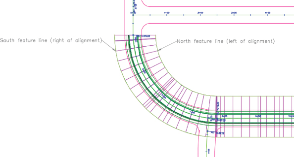
Figure 10.58 The corridor now uses the grading feature lines as width and elevation targets.
Once you've linked the corridor to these feature lines, any edits to the feature lines will be incorporated into the corridor model. You can establish this feature line at the beginning of the project and then make horizontal edits and elevation changes to perfect your design. The next few steps will lead you through making some changes to this feature line and then rebuilding the corridor to see the adjustments.
- Select the text that resides in the XRef. From the External Reference context tab Edit panel, click Open Reference.
This opens the external reference so you can modify the feature lines.
- Select one of the feature lines so that you can see its grips. Experiment with the feature lines by moving several grips.
- When you have edited several areas in the external reference file (
1009_XREF.dwgor1009_XREF_METRIC.dwg), save and close the drawing.After the external reference closes, you should be back in the corridor drawing. A message will appear in the lower-right corner of your screen indicating External Reference File Has Changed.
- In the bubble message, click the link to reload
1009_XREF.dwg(for metric users,1009_XREF_METRIC.dwg). - Press Esc to deselect, and then select the corridor. From the Corridor contextual tab Modify Corridor panel, click Rebuild Corridor.
The corridor will rebuild to reflect the changes to the target feature lines.
See 1009_FeatureLineTarget_FINISHED.dwg (1009_FeatureLineTarget_METRIC_FINISHED.dwg) to view a completed version of this exercise.
Edits to targets—whether they're feature lines, alignments, profiles, or other Civil 3D objects—drive changes to the corridor model, which in turn drives changes to any corridor surfaces, sections, section views, associated labels, and other objects that are dependent on the corridor model.
Tackling Roundabouts: the Mount Everest of Corridors
If you really understand what went on earlier in this chapter, you are almost ready for roundabout design. You may want to wait to tackle your first roundabout until after reading Chapter 14, “Grading.”
The same concepts apply to a roundabout as for a standard road junction, but you will have several more regions, baselines, and corresponding profiles.
The following sections will help you prepare files for roundabout design. We will not take you through every detail of corridor creation, but once you master the topics of intersection design, a roundabout is an extension of the same concepts.
A roundabout is best done in several corridors:
- Preliminary Corridor for Circulatory Road This is a corridor used to determine the elevations of the approach road profiles. The circular portion of the roadway will set the elevations for all of the alignments leading into it. Using similar techniques to those used earlier in the chapter, you create a corridor surface from this corridor and use it as a tie-in for approach road profiles.
- Main Corridor with Approaches and Circulatory Road This corridor is the main part of your design. You will spend lots of time in the corridor properties tweaking stations, adding baselines and regions, and targeting the appropriate locations.
- Curb Island Corridors (Optional) There are many different philosophies about the best way to show curb islands. If showing them in a section is not important, you can omit this altogether. Some people prefer to use grading feature lines (as discussed in Chapter 14). In the following sections, you will go “all out” and use the dynamic capabilities of the corridor model to make curb islands.
Drainage First
Based on your existing ground surface, determine the general direction that you want water to flow away from the center of the roundabout. Use grading tools and a feature line to create the general drainage direction of the roundabout.
Chapter 14 will go into much more depth on creating grading. You will certainly want to have an understanding of grading basics before you tackle a roundabout.
Create a feature line that represents the highest elevations. In the example shown in Figure 10.59, the feature line slopes downward and acts as a ridge to separate water flow. The grading tools are then used to create grading objects and a corresponding surface model called Roundabout Grading.
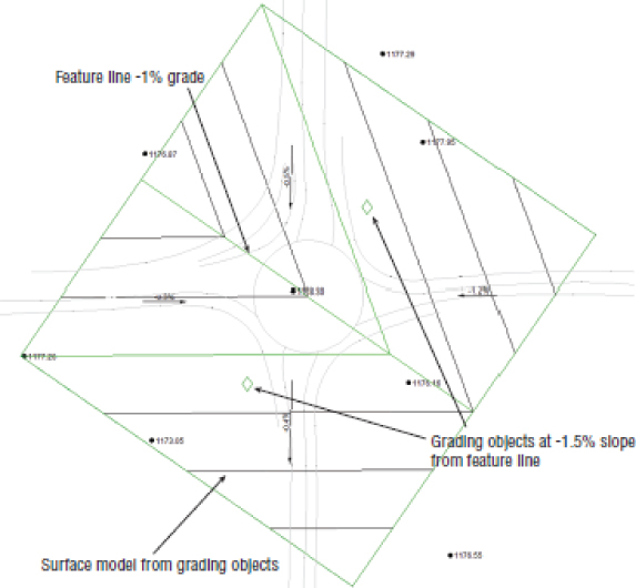
Figure 10.59 Feature lines and grading create a preliminary surface to ensure proper drainage through the roundabout.
The Roundabout Grading surface will be the basis for your profile elevations through the rest of the design process.
Roundabout Alignments
Roundabouts need alignments to guide the design for the same reasons that an intersection needs them. Alignments will be baselines and targets for the approaches and rotary. Create alignments manually with the tools you learned to use earlier in this chapter, or start with the handy roundabout layout tool.
The roundabout layout tool creates horizontal data based on the location of the center of the roundabout and the approach alignments.
In the exercise that follows, you will create the Civil 3D alignments needed to create a roundabout:
- Open the
1011_RoundaboutLayout.dwg(1011_RoundaboutLayout_METRIC.dwg) file, which you can download from this book's web page. - From the Home tab Create Design panel, select Intersections Create Roundabout, as shown in Figure 10.60.
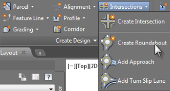
Figure 10.60 Access the Create Roundabout tool from the Home tab.
- At the
Specify roundabout center point:prompt, use your Intersection Osnap to select the point where the alignments intersect.The alignments leading into the roundabout are often referred to as approaches.
- At the
Select approach road:prompt, select all four alignments leading into the roundabout, and press ↵ when you have finished.You now see the Create Roundabout – Circulatory Road page of the wizard, shown in Figure 10.61.
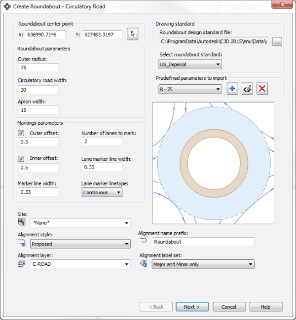
Figure 10.61 The first roundabout layout screen for designing the main circulatory road
- Verify that you are using the correct standards for your units. Click the ellipsis next to the Roundabout Design Standard File field, and verify that you are using the correct XML standards file. Imperial users should be using
Autodesk Civil 3D Imperial Roundabouts Presets.xml. Metric users should be usingAutodesk Civil 3D Metric Roundabouts Presets.xml.- If Roundabout Design Standard File is set correctly, click Cancel and continue to step 6.
- If it is not set correctly, browse to the
C:ProgramDataAutodeskC3D 2015enuDataCorridor Design Standardsfolder. Browse to either the Imperial or Metric units folder and select the correct roundabout presets XML file. Click Open to return to the Create Roundabout dialog.
- From the Predefined Parameters To Import drop-down, choose R = 75 (Rg = 25m).
This will be the radius from the center of the roundabout to the outermost circular edge of pavement. This will also adjust other settings in the dialog.
- Set Alignment Layer to C-ROAD and Alignment Label Set to Major And Minor Only. Click Next.
Now, you'll design the approach road exit and entry geometry. The options in the Create Roundabout – Approach Roads page of the wizard (see Figure 10.62) can be set independently for each approach, or you can click Apply To All, which will set the geometry for all four approaches.
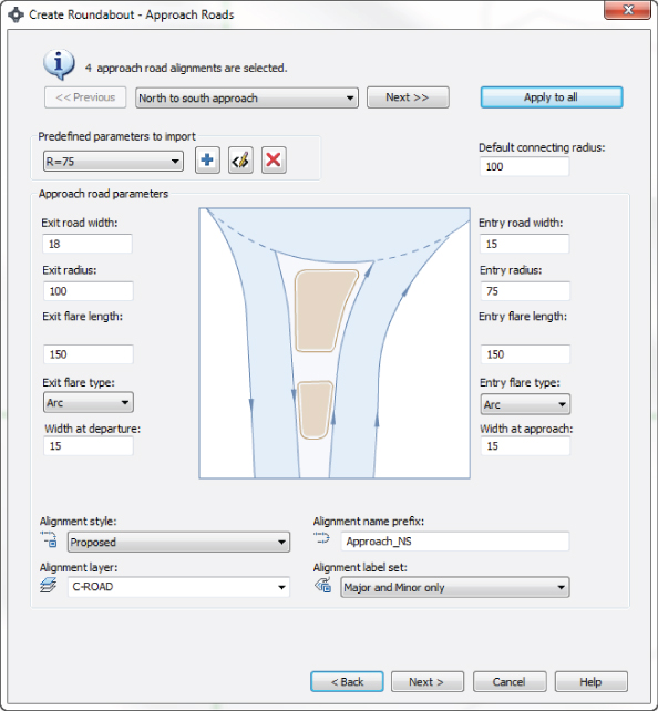
Figure 10.62 Approach road widths at entry and exit
- On the Create Roundabout – Approach Road page, do the following:
- Set Predefined Parameters To Import to R = 75 (Rg = 25m).
- Change the alignment layer to C-ROAD. Hint: You can type in the layer name or pick it from the drop-down.
- For Alignment Label Set, choose Major And Minor Only.
- Leave all other settings at their defaults.
- Click the Apply To All button, and click Next.
- In the Create Roundabout – Islands screen (see Figure 10.63), again set Predefined Parameters To Import to R = 75 (Rg = 25m).
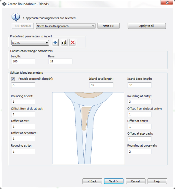
Figure 10.63 Roundabout Islands parameters
- Click Apply To All, and then click Next.
The final screen of the Create Roundabout Wizard deals with pavement markings and signage. Notice that you can specify your own blocks for the signs that will be placed in this process.
Everything created in this last step is an AutoCAD polyline or block. The polylines have a global width set to indicate pavement marking thicknesses. These thicknesses are set in the Markings And Signs page (Figure 10.64).
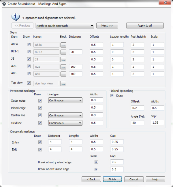
Figure 10.64 Pavement markings galore!
- Leave all defaults in the Create Roundabout – Markings And Signs page (Figure 10.64), and click Finish.
Your roundabout should resemble Figure 10.65. Since standards vary by region, the metric drawing will have slightly different default pavement markings.
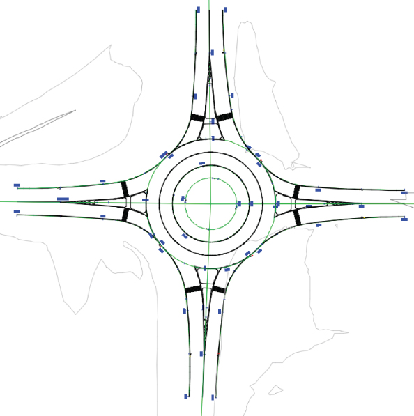
Figure 10.65 Completed roundabout alignment layout
Finally, you will add a turn lane in the NW quadrant of the roundabout. When you're creating slip turn lanes, remember that the turn radius must be large enough to fillet the exit and entry roads without overlapping the other alignments.
When selecting the approach entry and exit alignments, you need to click the shorter approach alignments created by Civil 3D rather than the original approach road. For this reason, the exercise has you select inside the islands, just to be sure.
- From the Home tab Create Design panel, select Intersections Add Turn Slip Lane.
- When prompted to select the entry approach, select the north approach alignment inside the curb island.
- When prompted for the exit approach, select the west approach alignment inside the curb island, as shown in Figure 10.66.
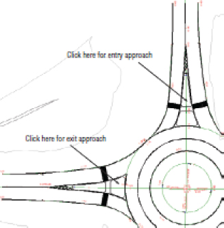
Figure 10.66 Entry and exit approach alignments for the slip lane
- In the Draw Slip Lane dialog shown in Figure 10.67, set the lane width to 14′ (4 m) and the radius to 150′ (45 m).
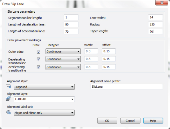
Figure 10.67 Adding a slip lane
- For Alignment Layer, choose C-ROAD, and for Alignment Label Set, choose Major And Minor Only. Click OK.
Your roundabout will now look like Figure 10.68.
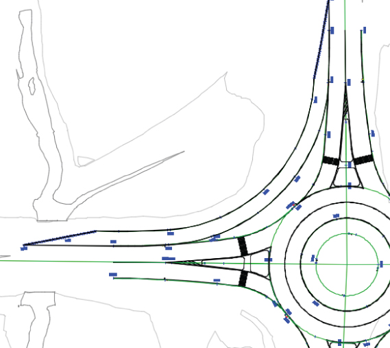
Figure 10.68 The completed slip lane alignments
- Save and close the drawing.
The completed files, 1011_RoundaboutLayout_FINISHED.dwg and 1011_RoundaboutLayout_METRIC_FINISHED.dwg, are available for your review if desired.
You now have all the alignments you need to start your roundabout design. At this point, you can add geometry to the alignments and modify what Civil 3D has created for you.
The horizontal layout is complete, but the roundabout design is far from done. No vertical data has been created; that is up to you.
This is as far as we will take you in this book in regard to building a roundabout step by tedious step. Rest assured, however, that if you have truly mastered corridors, the technique for completing a roundabout is similar to that used for any intersection.
The remainder of this chapter gives you an overview of how to accomplish the rest on your own.
Center Design
All profiles need to meet at the elevations inside the traveled way in the circular pavement area of the roundabout. Therefore, the main circle design comes first.
To see an example of a completed roundabout corridor, open the drawing 1011_RoundaboutExample_FINISHED.dwg or 1011_RoundaboutExample_METRIC_FINISHED.dwg. Use these examples as a guide to “reverse engineer” your own roundabouts when you've mastered other forms of intersections.
You can use any of the circular alignments created by Civil 3D as the basis for this step, as long as your assembly works with the design. Remember to make note of which direction the alignment goes, to ensure that the assembly you create is not backward.
Extract profiles for the main circle design from the Existing Intersection and Roundabout Grading surfaces, as shown in Figure 10.69.
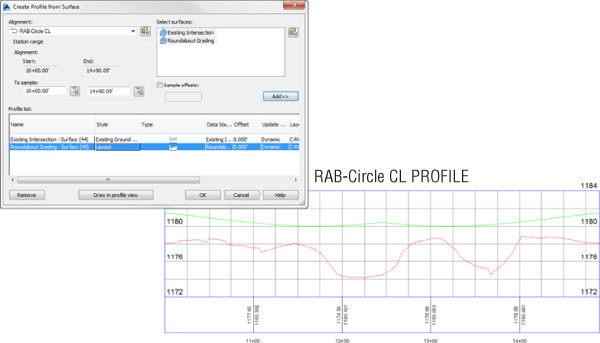
Figure 10.69 Extract surface profiles around the main circular alignment.
The assembly you create for this preliminary design will also be used in the main design. Decide which alignment will be used as the circular design basis, and create an assembly based on your alignment location and desired geometry, as shown in Figure 10.70.
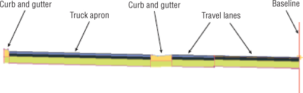
Figure 10.70 Center assembly for roundabout
This assembly can be used in several steps of the process. First, it is used in a preliminary corridor called RAB MAIN. It can also be recycled to be the centerpiece of your main corridor. In the example, the main circle alignment created by Civil 3D, Roundabout_OUTER_EDGE, was used as the baseline for this initial corridor. There are no targets or frequencies set in this corridor. Like the cul-de-sac example earlier in this chapter, this is a preliminary corridor, used to ensure that profiles from the approach roads tie in at the correct elevations.
In the example drawings, a Top link surface was created from the RAB MAIN corridor. At this point, the roundabout will resemble Figure 10.71.
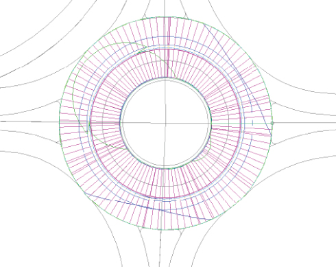
Figure 10.71 Preliminary center corridor and surface
Profiles for All
You have all the preliminary surfaces in place, and you have all the alignments you need, so it is time to extract profiles from your various surfaces.
In the 1011_RoundaboutExample_FINISHED.dwg and 1011_RoundaboutExample_METRIC_FINISHED.dwg files, the surface profiles for all the approach alignments were created by sampling the existing ground, drainage surface, and preliminary RAB MAIN corridor surface. These profiles will look something like Figure 10.72.
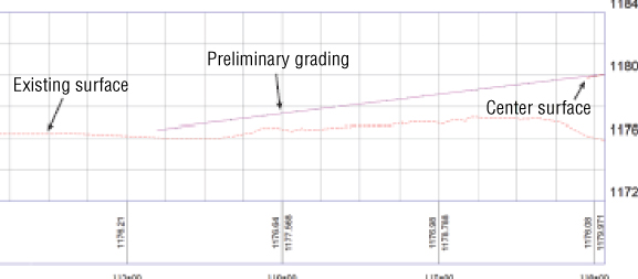
Figure 10.72 Surface profiles needed for design
When you create your design, you will see all your design considerations in the profile views. No matter how you decide to tie into existing ground and slope upward toward the surface, your design must tie into the preliminary center surface, as shown in Figure 10.73.
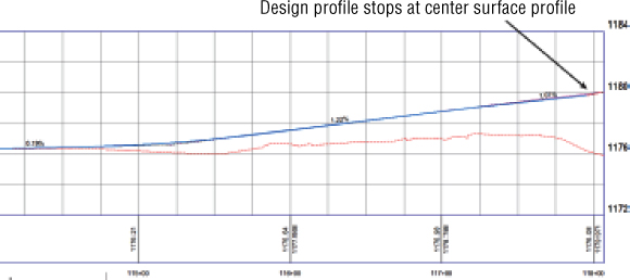
Figure 10.73 Design profiles must tie into the center.
Use techniques you learned earlier in this chapter to assist you. Labels are an especially valuable tool for roundabouts. Keep your profile views organized because you will have at least three for each approach. If you have a slip turn lane, you will have a profile for that as well.
Tie It All Together
Stretch your legs and go for more coffee. It is time to put this thing together into a completed corridor. When you model the corridor initially, ignore curb islands—you will add them as individual corridors in a later step.
A simple roundabout can be completed using as few as three assemblies. In our example, however, the slip turn lane necessitates a total of four assemblies. In addition to the RAB Main assembly you saw in Figure 10.70, you will need three more assemblies, as shown in Figure 10.74.
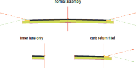
Figure 10.74 Assemblies needed for the main roundabout corridor
These assemblies will be tied to the EOP alignments and profiles as baselines, similar to a traditional intersection. Each quadrant of the roundabout will target at least two alignments and profiles, as shown in Figure 10.75.
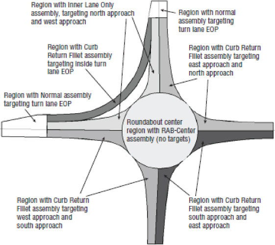
Figure 10.75 Roundabout corridor regions and targets
Keep in mind the direction of your alignments. If you build the corridor in stages, check the corridor periodically to make sure it is building correctly.
Create a corridor surface from your completed roundabout lanes. You will likely have to use the Add Interactively tool to add the boundary correctly.
Finishing Touches
The median islands are the last parts to go on the corridor. You can create them using simple grading objects, but since this is a book about mastering skills, and this is a chapter about corridors, you should examine the dynamic way.
Create a simple assembly containing the curb and gutter for the curb islands. This will be the assembly that you use with the median corridors (Figure 10.76).

Figure 10.76 Simple assembly containing just the curb and gutter on the median islands
Each median island will need its own alignment. Take note of the direction of the alignments to make sure they are compatible with the curb island assembly. If necessary, change the direction of the alignments using the Reverse Direction tool in the Modify panel of the contextual ribbon tab. Figure 10.77 shows the bypass island and north island with directions.
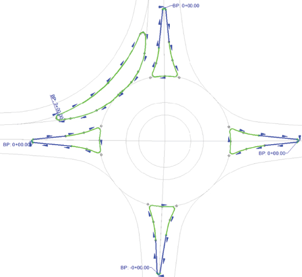
Figure 10.77 Several median island alignments with direction shown
The good news is that the elevation data for the medians is already complete. Your main corridor's surface will act as the profile for each individual median. This also means that once the curb return corridors are created, they will be dynamic to the main corridor. After these little corridors are created and surface model information has been obtained, you can set them to Rebuild – Automatic and forget all about them.
Extract a profile for all the curb return alignments from the Top link surface model from the main roundabout corridor, as shown in Figure 10.78. You do not need to see this profile in a view, so you can click OK to extract.
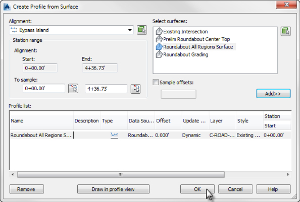
Figure 10.78 Extract the profile for medians from your main : roundabout surface.
When the design roundabout corridors are complete and surfaces are made, the next step is to merge the surfaces. Create a final surface model and paste the main roundabout design in first. After the main corridor is pasted in, paste the smaller median corridor surfaces, as shown in Figure 10.79. The center median is already taken care of by the first baseline.
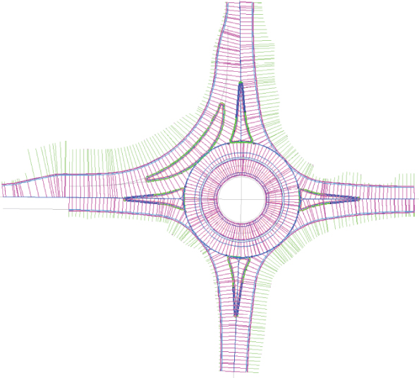
Figure 10.79 The completed roundabout
Your next step is to use the corridor fine-tuning techniques you learned earlier in this chapter to ensure that your grades are correct and the design is correct. To see an example of a completed corridor using these steps, take a look at 1011_RoundaboutExample_FINISHED.dwg (1011_RoundaboutExample_FINISHED_METRIC.dwg), which you can download from this book's web page.
The Bottom Line
- Create corridors with non-centerline baselines. Although for simple corridors you may think of a baseline as a road centerline, other elements of a road design can be used as a baseline. In the case of a cul-de-sac, the EOP, the top of curb, or any other appropriate feature can be converted to an alignment and profile and used as a baseline.
- Master It Open the
MasterIt1001.dwg(MasterIt1001_METRIC.dwg) file, which you can download from www.sybex.com/go/masteringcivil3d2015. Add the cul-de-sac alignment and profile to the corridor as a baseline. Create a region under this baseline that applies the Intersection Typical assembly.
- Master It Open the
- Add alignment and profile targets to a region for a cul-de-sac. Adding a baseline isn't always enough. Some corridor models require the use of targets. In the case of a cul-de-sac, the lane elevations are often driven by the cul-de-sac centerline alignment and profile.
- Master It Continue working in the
MasterIt1001.dwg(MasterIt1001_METRIC.dwg) file. You need to have completed the previous exercise before continuing. Add the Second Road alignment and Second Road FG profile as targets to the cul-de-sac region. Adjust Assembly Application Frequency to 5′ (1 m) for tangents and curves.
- Master It Continue working in the
- Create a surface from a corridor and add a boundary. Every good surface needs a boundary to prevent bad triangulation. Bad triangulation creates inaccurate contours and can throw off volume calculations later in the process. Civil 3D provides several tools for creating corridor surface boundaries, including an Interactive Boundary tool.
- Master It You need to have completed the previous exercise before continuing. Keep working in the
MasterIt1001.dwg(MasterIt1001_METRIC.dwg) file. Create an interactive corridor surface boundary for the entire corridor model.
- Master It You need to have completed the previous exercise before continuing. Keep working in the