
Chapter 12
Cross Sections and Mass Haul
Cross sections are used in the Autodesk® AutoCAD® Civil 3D® program to allow the user to have a graphic confirmation of design intent as well as to calculate the quantities of materials used in a design. All that is needed for section creation is an alignment and a surface. Other objects, such as pipes, structures, and corridor components, can be sampled in a sample line group, which is used to create the graphical section displayed in a section view. These section views and sections remain dynamic throughout the design process, reflecting any changes made to the sampled information. The result is a plot-worthy set of section views and accurate end area volume information.
In this chapter, you will learn to
- Create sample lines
- Create section views
- Define and compute materials
- Generate volume reports
Section Workflow
When the time comes that you wish to see how the information along your alignment will appear plotted, you can create sample lines. If your goal is to show your completed design, at this point you should have a completed corridor, corridor top surface, and corridor datum surface.
Comparing Sample Lines and Frequency Lines
Sample lines are created at any stations where you wish to create a section view. Sample lines are also used to compute end area volumes.
A common point of confusion with new users is the difference between frequency lines and sample lines. Table 12.1 explains the differences.
Table 12.1 Sample lines vs. frequency lines
| Sample lines & section views | Frequency lines & Section Editor |
| Sample lines can be created without a corridor present (e.g., when you wish to see existing surface sections along the alignment). | Frequency lines are only part of a corridor. |
| Sample lines occur at any station where a section view or end area is needed. | Frequency lines occur anywhere the design needs to be calculated or modified (e.g., at certain station intervals, a driveway). |
| Sample lines are used for end area volume computation. | Frequency lines are used to apply assembly calculations to the design (e.g., locating slope-intercept). |
| Sample lines can be skewed at an angle other than 90º from the baseline. | Frequency lines are always perpendicular to the baseline. |
| Sample line swath width is usually uniform and dependent on user plotting needs. | Frequency lines' length from baseline depends on assembly and will vary from station to station. |
| Section views are read-only reflections of the design. | Design can be modified in the Section Editor at each frequency line. |
| Section views are readily adapted to plotting. | Plotting should never occur from the Section Editor. |
When you create your sample line group, you will have the option to sample any surface in your drawing, including corridor surfaces, the corridor assembly itself, and pipes. The sections are then sampled along the alignment with the left and right swath widths specified and at the intervals specified. After you create sample lines, you can create section views or define materials for end area volume calculations.
Creating Sample Lines
A sample line is a powerful tool needed for both section view creation and end area material computations. Sample lines are created in batches and stored in sample line groups. A sample line group is always associated with an alignment and can be found under the associated alignment in Prospector, as shown in Figure 12.1.
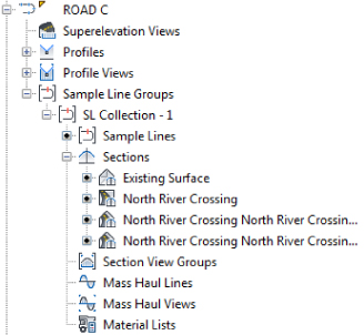
Figure 12.1 A view of Prospector; sample lines are stored in sample line groups and are dependent on an alignment.
You can also see in Figure 12.1 that quite a few additional items are dependent on sample lines, such as sections, section view groups, mass haul lines, mass haul views, and material lists. If you click a sample line, you will see that it has three types of grips, as shown in Figure 12.2.
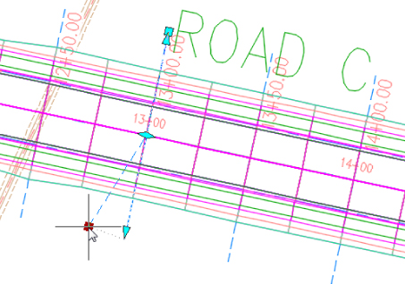
Figure 12.2 The three grips on a typical sample line
The grips are intended for changes to a sample line that cannot be accomplished through the sample line group properties. The diamond-shaped grip at the alignment location will allow you to slide the sample line to a different station. The triangular grips at the ends of a sample line allow you to extend the sample line swath width while maintaining its angle in relation to the alignment. The square grips on the sample line will allow you to change the length and angle of the sample line. If you have used the square grip to skew a sample line but wish to return it to its original perpendicular state, select the sample line, right-click with the mouse, and then click Make Orthogonal from the menu, as shown in Figure 12.3. Note that this command is available only from the context menu, not in the ribbon tab.
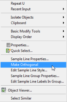
Figure 12.3 Removing the skew with the Make Orthogonal command
To create a sample line group, change to the Home tab ![]() Profile & Section Views panel and choose Sample Lines. After you select the appropriate alignment, the Create Sample Line Group dialog, shown in Figure 12.4, will appear. You should name the sample line group and verify the sample line and label styles.
Profile & Section Views panel and choose Sample Lines. After you select the appropriate alignment, the Create Sample Line Group dialog, shown in Figure 12.4, will appear. You should name the sample line group and verify the sample line and label styles.
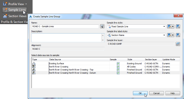
Figure 12.4 Click the Sample Lines icon to open the Create Sample Line Group dialog.
Every source object that is available will be displayed at the bottom of this box. If you wish to omit specific data from the section view, you can clear the check box. Set the applicable style for each item by clicking in the column to the right of the object. The section layer should be preset as specified in your template Object Layers settings.
Once you've selected the sample data and clicked OK, the Sample Line Tools toolbar that shows in the background will become active (Figure 12.5).
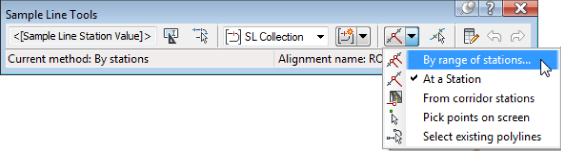
Figure 12.5 From the Sample Line Tools toolbar, choose By Range Of Stations.
The By Range Of Stations option is used most often. You can use At A Station to create one sample line at a specific station. From Corridor Stations will insert a sample line at the same locations as corridor frequency stations. Pick Points On Screen allows you to pick any two (or more) points to define a sample line. This option can be useful in special situations, such as sampling a pipe on a skew or cross sections for drainage area calculations. The last option, Select Existing Polylines, lets you define sample lines from existing polylines. Like Pick Points On Screen, this tool is useful in the case of cross sections for drainage area calculations.
To define sample lines, you need to specify a few settings. Figure 12.6 shows these settings in the Create Sample Lines - By Station Range dialog.
- Station Range Station Range controls where on your alignment sample lines are created. By default, the dialog picks up the start and end station of the alignment. Change the station range by changing From Alignment Start or To Alignment End to False and setting the desired stations.
- Left/Right Swath Width Swath width is the offset from the alignment along which you create sample lines. When using sample lines for end area volume calculations, be sure that the swath width is large enough to encompass the design but not so large that they overlap in curve areas. You can change the Snap To An Alignment option to True if you wish to force your sample lines to stop at an alignment that is not a constant offset from the centerline.
- Sampling Increments Sampling Increments allows you to choose the interval at which sample lines are created. Notice that you can control the sample line interval separately along tangents, curves, and spirals.
- Additional Sample Controls Additional Sample Controls adds a sample line at the beginning, end, and other special stations, such as horizontal geometry (PC, PT, and so on) and superelevation critical stations.
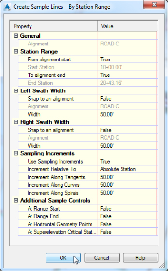
Figure 12.6 Create Sample Lines – By Station Range dialog
![]() In the following exercise, you'll create sample lines for ROAD C alignment:
In the following exercise, you'll create sample lines for ROAD C alignment:
- Open the
1201_SampleLines.dwg(1201_SampleLines_METRIC.dwg) file, which you can download from this book's web page at www.sybex.com/go/masteringcivil3d2015.  From the Home tab
  Profile & Section Views panel, choose Sample Lines.
- At the
Select an alignment, <or press enter key to select from list>:prompt, press ↵ to display the Select Alignment dialog. - Select the ROAD C alignment and click OK.
The Create Sample Line Group dialog opens.
- In the Create Sample Line Group dialog, follow these steps:
- Name the group ROAD C - Sample Lines.
- Set Existing Surface to the Existing Ground style, if not already set, by selecting that style from the Style column. (Hint: The first click will activate the cell, and the second click will give you the list of styles.)
- Set the style for both the Top and Datum corridor surfaces to Finished Ground.
The column is too narrow to view the full names of the items, so to see the name of the item, pause your cursor over the name or expand the column.
- Set the corridor North River Crossing style to All Codes.
- Leave the default settings for Sample Line Style and Sample Line Label Style.
- When your dialog looks similar to Figure 12.4 (your sampled items may be listed in a different order), click OK.
 On the Sample Line Tools toolbar, click the Sample Line Creation Methods drop-down arrow and then choose By Range Of Stations.
- In the Create Sample Lines – By Station Range dialog, leave the swath widths and sampling increments at their defaults (this will be 50.00′ for Imperial units and 20.00 m for metric units).
- Make sure that both the At Range Start and At Range End options are set to False, as shown earlier in Figure 12.6.
- Click OK, and press ↵ to end the command.
- If you receive a Panorama view telling you that your corridor is out of date and may require rebuilding, dismiss it by clicking the green check box.
You should now have dashed lines at even station intervals; these are your new sample lines.
- Save the drawing for use in the next exercise.
Check your completed drawings at this stage against 1201_SampleLines_A.dwg or 1201_SampleLines_A_METRIC.dwg if desired.
Editing the Swath Width of a Sample Line Group
There may come a time when you need to show information outside the limits of your section views or not show as much information. To edit the width of a section view, you will have to change the swath width of a sample line group. These sample lines can be edited manually on an individual basis, or you can edit the entire group at once.
In this exercise, you'll edit the widths of an entire sample line group.
- Continue working on the
1201_SampleLines.dwg(1201_SampleLines_METRIC.dwg) file or open1201_SampleLines_A.dwg(1201_SampleLines_A_METRIC.dwg). - Select a sample line.
 From the Sample Line contextual tab Modify panel, click Group Properties.
- Switch to the Sample Lines tab.
- Click to select the first sample line in the listing at station 0+00.00 (0+000.00).
- Scroll down to the bottom of the list.
- While holding the Shift key, select the last station in the listing. This will highlight all rows.
- Click your mouse in the Left Offset column and change it to 100′ (30 m). Press ↵ to complete the edit.
The left offsets will change in the listing. If you have a long list of sample lines in a project, it may take a moment to update.
- With all of the rows still highlighted, make the same change to the Right Offset column.
- Click OK.
- After a moment, the sample lines will resize to reflect your change. The Event Viewer panorama might appear.
- Save the drawing. Check your completed drawings against
1201_SampleLines_FINISHED.dwgor1201_SampleLines_METRIC_FINISHED.dwgif desired.
Creating Section Views
Once the sample line group is created, it is time to create views. You can create a single view or many views arranged together (Figure 12.7).
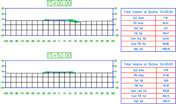
Figure 12.7 Section views arranged to plot by page
A section view is a reflection of the design and can be used for plotting purposes. No edits to the corridor, surface, or other design elements can be made from a section view. The view contains horizontal and vertical grids, tick marks for axis annotation, the axis annotation itself, and a title. Views can also be configured to show horizontal geometry, such as the centerline of the section, edges of pavement, and right of way. Tables displaying end areas or volumes can also be shown with the sections.
Creating a Single-Section View
![]() There are occasions when all section views are not needed. In these situations, a single-section view can be created. In this exercise, you'll create a single-section view of station 15 + 00.00 (0+460.00 for metric users) from sample lines:
There are occasions when all section views are not needed. In these situations, a single-section view can be created. In this exercise, you'll create a single-section view of station 15 + 00.00 (0+460.00 for metric users) from sample lines:
- Open the
1202_SectionViews.dwg(1202_SectionViews_METRIC.dwg) file, which you can download from this book's web page.You will want to switch to this drawing because there are a few steps completed for you that you will learn about later in the chapter.
- Select the sample line at 15+00.00 (0+460.00 for metric users).
 From the Sample Line contextual tab Launch Pad panel, choose Create Section View Create Section View.
- Verify that your alignment and sample line group name are correct on the General page of the wizard, shown in Figure 12.8.

Figure 12.8 The General page of the Create Section View Wizard
You can navigate from one page to another by either clicking Next at the bottom of the screen or clicking the links on the left side of the screen.
- Click Next to view the Offset Range page.
The top of Figure 12.9 shows the Offset Range page, which should match your sample line swath width. In this case, you will leave this set to Automatic. No action is needed on the Offset Range page.
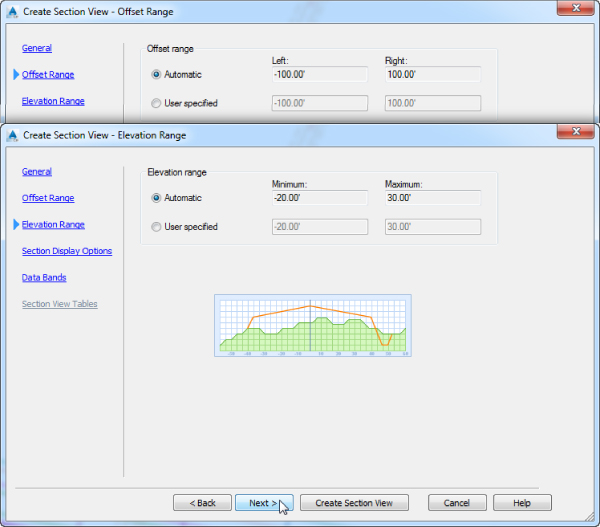
Figure 12.9 The Offset Range page (top) and Elevation Range page (bottom) of the Create Section View Wizard
- Click Next to view the Elevation Range page.
The bottom of Figure 12.9 shows the Elevation Range page. The values shown here are taken from your design max and min elevations. In this case, and in most cases, you will leave this set to Automatic. No action is needed on the Elevation Range page.
- Click Next to view the Section Display Options page. Change all three surface label styles to _No Labels by clicking in the Label Set column for each surface item.
The fourth page contains the section display options, as shown in Figure 12.10. This page reflects the styles and data you selected when creating your sample lines. If you forgot to set a style or wish to omit additional data, you can change your options here.
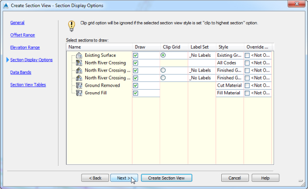
Figure 12.10 The Section Display Options page of the Create Section View Wizard
- Click Next to view the Data Bands page.
The fifth page, shown in Figure 12.11, lets you specify the data band options. Here, you can select band sets to add to the section view, pick the location of the band, and choose the surfaces to be referenced in the bands. The data bands used in this example show only offset distance (rather than offset and elevation), and therefore no action is needed on the Data Bands page.
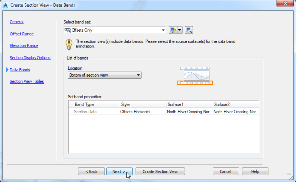
Figure 12.11 The Data Bands page of the Create Section View Wizard
- Click Next to view the Section View Tables page.
The sixth and last page, shown in Figure 12.12, is where you set up the section view tables. Note that this screen will be available only if you have already computed materials for the sample line group. On this page, you can select the type of table and the table style and select the position of the table relative to the section view. The graphic on the lower-right side of the window will help to illustrate the table placement and changes as you update these settings.
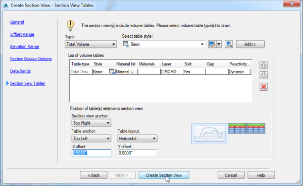
Figure 12.12 The Section View Tables page of the Create Section View Wizard
- With the table type set to Total Volume and Select Table Style set to Basic, click Add.
As shown in Figure 12.12, you will have a row of data indicating that a material table will come in to the right of your view. Make sure that the X Offset is set to 0.5 (10 for metric users).
- Click the Create Section View button.
- Pick any point in the drawing area to place your section view.
- Examine your section view.
The display should resemble Figure 12.13.
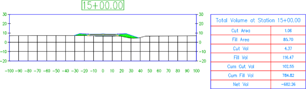
Figure 12.13 The finished section view
- Save the drawing for use in the next exercise.
Check your completed drawings at this stage against 1201_SectionViews_A.dwg or 1201_SectionViews_A_METRIC.dwg if desired.
Creating Multiple Section Views
Section views belong in packs. In the exercise that follows, you will create section views intended to plot together on a sheet:
- Continue working in
1202_SectionViews.dwg(1202_SectionViews_METRIC.dwg) or open1202_SectionViews_A.dwg(1201_SectionViews_A_METRIC.dwg). You do not need to have completed the previous exercise to continue. - Change your drawing scale to 1″ = 20′ (1:500 for metric users) from the lower-right corner of the drawing window, and select any sample line.
- From the Sample Line contextual tab Launch Pad panel, choose Create Section View Create Multiple Section Views.
Alternatively, you can access this tool from the Home tab
Profile & Section Views panel Section Views Create Multiple Views. - On the General page, set the Section View Style option to Road Section, if not already set, and leave all the other settings at the default. Click Next.
- On the Section Placement page, click the ellipsis button next to the path for Template For Cross Section Sheet.
- From the default cross section sheet template, select ARCH D Section 20 Scale (ISO A1 Section 1 to 500 for metric users), as shown in Figure 12.14, and click OK.
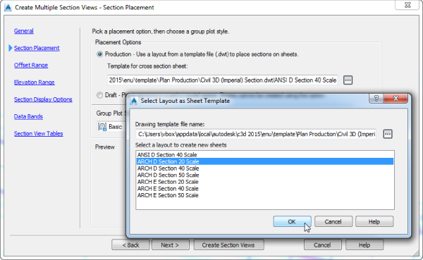
Figure 12.14 When you're creating multiple views, the scale and spacing of the final product depend on layouts from sheet templates.
The Civil 3D default cross section template should be
Civil 3D (Imperial) Section.dwtorCivil 3D (Metric) Section.dwt. Each scale listed in the dialog box (Figure 12.14) relates to a layout tab in the section template file. You can also set up your own templates based on these layouts, but it is important to note that the viewports set for the sections must be assigned that type in the Viewport object AutoCAD properties. - Leave Group Plot Style set to Basic, and click Next.
You did not see the Create Multiple Section Views - Section Placement page, shown in Figure 12.14, when placing a single view. Setting the Production radio button allows you to use the Create Section Sheets tool from the Output tab. The Draft option forces Civil 3D to behave like version 2010 and prior. Do not use the Draft option if you intend to run the Create Section Sheets command with the section views.
Group Plot Style controls how the views are arranged on a page. In this example, the grid will come from the group plot style rather than the section view style.
You can skip the rest of the wizard because you will keep the default input for the remainder of the settings.
- Click the Create Section Views button.
- Click anywhere off to the right of the graphic to place the views.
You should see views arranged on the screen (Figure 12.15). Metric users will see two pages of section views, and Imperial unit users will see three pages of section views. Notice that the scale chosen in the Select Layout As Sheet dialog box matches the annotative scale of the drawing, creating a neat, coherent set of section views.
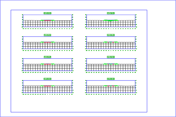
Figure 12.15 One of the pages of cross-section views
- Save the drawing for use in the next exercise.
Check your completed drawings at this stage against 1202_SectionViews_B.dwg or 1202_SectionViews_B_METRIC.dwg if desired.
Section Views and Annotation Scale
In the last section, you created section views using a cross-section sheet template. You chose a scale for the section sheet layout at the same time that you picked a page size. Coincidentally, the scale you used in the exercise was already set as the annotation scale. Since both scales agreed with each other, everything came out nicely.
Depending on what portion of the design you are working on, the scale of the sections and the scale you are comfortable working with may not agree. Additionally, you may just forget to set the scale ahead of placing section views.
Ideally, your section views and their sheets should be in a drawing separate from the corridor and the rest of the design. In Chapter 16, “Advanced Workflows,” you will learn how to do this using data shortcuts.
It is helpful to learn how to work with annotation scale and section views. In the following exercise, you will go through a brief lesson in reorganizing sections:
- If you completed the previous exercise, continue working in your open file; otherwise, open
1202_SectionViews_B.dwg(1202_SectionViews_B_METRIC.dwg). - Select the Annotation scale in the lower-right portion of the screen.
- Change the scale to 1″=10′ (1:250 mm).
- The views probably look pretty funky—and not in a good way. The page has gotten smaller, but the views have not updated.
- Select any section view by clicking on the station value.
 From the Section View contextual tab Modify View panel, click Update Group Layout.
- Save and close the drawing.
- The views should now be reorganized to a better-looking state.
Check your completed drawings against 1202_SectionViews_FINISHED.dwg or 1202_SectionViews_METRIC_FINISHED.dwg if desired.
Calculating and Reporting Volumes
Once alignments are sampled, volumes can be calculated from the sampled surface or from the corridor section shape. These volumes are calculated in a materials list and can be displayed as a label on each section view or in an overall volume table, as shown in Figure 12.16.
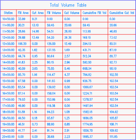
Figure 12.16 A total volume table inserted into the drawing
The volumes can also be displayed in an XML report, as shown in Figure 12.17.
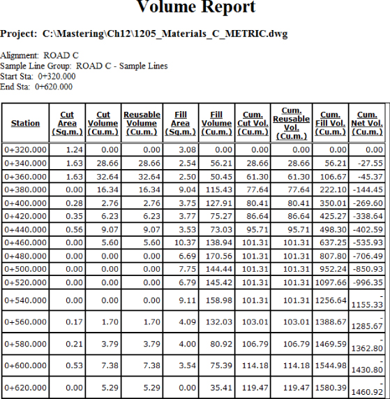
Figure 12.17 A total volume XML report shown in the browser
Once a materials list is created, it can be edited to include more materials or to make modifications to the existing materials. For example, soil expansion (fluff or swell) and shrinkage factors can be entered to make the volumes more accurately match the true field conditions. This can make cost estimates more accurate, which can result in fewer surprises during the construction phase of any given project.
Computing Materials
![]() Materials can be created from surfaces or from corridor shapes. Surfaces are great for earthwork because you can add cut or fill factors to the materials, whereas corridor shapes are great for determining quantities of asphalt or concrete. In this exercise, you practice calculating earthwork quantities for the ROAD C corridor:
Materials can be created from surfaces or from corridor shapes. Surfaces are great for earthwork because you can add cut or fill factors to the materials, whereas corridor shapes are great for determining quantities of asphalt or concrete. In this exercise, you practice calculating earthwork quantities for the ROAD C corridor:
- Open the
1205_Materials.dwg(1205_Materials_METRIC.dwg) file, which you can download from this book's web page.  From the Analyze tab Volumes And Materials panel, choose Compute Materials.
The Select A Sample Line Group dialog appears.
- Select the ROAD C alignment and the ROAD C - Sample Lines group, and click OK.
The Compute Materials dialog appears.
- In the Quantity Takeoff Criteria drop-down box, select Earthworks from the drop-down menu.
- Click the Object Name cell for the Existing Ground surface, and select Existing Surface from the drop-down menu.
- Click the Object Name cell for the Datum surface, and select North River Crossing North River Crossing - Datum (this is the name of the corridor followed by the name of the surface) from the drop-down menu.
- Verify that your settings match those shown in Figure 12.18, and then click OK.
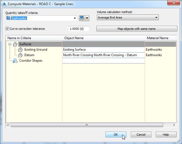
Figure 12.18 The settings for the Compute Materials dialog
Graphically, nothing will happen. However, in the background Civil 3D has computed material data.
- Save the drawing for use in the next exercise.
- Check your completed drawings at this stage against
1205_Materials_A.dwgor1205_Materials_A_METRIC.dwgif desired.
Creating a Volume Table in the Drawing
In the preceding exercise, materials were computed that represent the total dirt to be moved or used in the sample line group. In the next exercise, you insert a table into the drawing so you can inspect the volumes.
- If you completed the previous exercises, continue working in
1205_Materials.dwg(1205_Materials_METRIC.dwg); otherwise open1205_Materials_A.dwg(1205_Materials_A_METRIC.dwg).  From the Analyze tab Volumes And Materials panel, choose Total Volume Table.
- The Create Total Volume Table dialog appears.
- Verify that your settings match those shown in Figure 12.19.
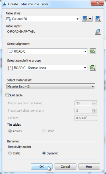
Figure 12.19 The Create Total Volume Table dialog settings
- Verify that Reactivity Mode at the bottom of the dialog is set to Dynamic.
- Clear the check box next to Split Table and click OK.
- Pick a point in the drawing to place the volume table.
- The table indicates a cumulative fill volume of 1896.91 cubic yards (1580.39 cubic meters) and a cumulative cut volume of 111.85 cubic yards (119.47 cubic meters).
- Save the drawing for use in the next exercise.
- Check your completed drawings at this stage against
1205_Materials_B.dwgor1205_Materials_B_METRIC.dwgif desired.
Adding Soil Factors to a Materials List
![]() Civil 3D allows for more accurate earthwork computations by providing entry of cut factors, fill factors, and refill factors.
Civil 3D allows for more accurate earthwork computations by providing entry of cut factors, fill factors, and refill factors.
- Cut Factor Sometimes known as expansion factor, or “fluff” factor, the cut factor is always expressed as a number greater than or equal to 1.0. Cut volume is multiplied by this value to determine the volume of soil after excavation has taken place. For example, soil that expands 5 percent after excavation would use a cut factor of 1.05.
- Fill Factor Commonly known as compaction factor, the fill factor is used to determine the volume of material after it has been mechanically compacted. Counter to most people's intuition, this value is also expressed as a value greater than or equal to 1.0. A material that compacts to 90 percent of its original volume would use a fill factor of 1.1. The fill volume is divided by the fill factor to determine the final amount of fill needed on a site.
- Refill Factor The refill factor dictates what amount of the cut material can be reused as fill. This value is expressed as a percentage of the cut volume (with cut factor applied). This factor is used only when the material quantity type is set to Cut And Refill.
In the following exercise, the materials need to be modified to bring them closer in line with true field numbers. For this exercise, the shrinkage factor will be assumed to be 80 percent, which is entered into Civil 3D as 1.2. The expansion on cut will be 115 percent, or, as entered into Civil 3D, 1.15. In addition to these numbers (which Civil 3D represents as cut factor for swell and fill factor for shrinkage), for this exercise, we assume a Refill Factor value of 1.00.
- If you completed the previous exercise, continue working in
1205_Materials.dwg(1205_Materials_METRIC.dwg); otherwise open1205_Materials_B.dwg(1205_Materials_B_METRIC.dwg). - From the Analyze tab Volumes And Materials panel, choose Compute Materials.
- The Select A Sample Line Group dialog appears.
- Select the ROAD C alignment and the ROAD C - Sample Lines group, and click OK.
- The Edit Material List dialog appears. We will use a different criteria that allows the input of the previously mentioned values.
- Click the Import Another Criteria button, and from the Select A Quantity Takeoff Criteria dialog select the Cut And Fill criteria and click OK.
- In the Compute Materials - ROAD C - Sample Lines dialog, click the <Click Here To Set All> cell and set the EG surface to Existing Surface. Click the same cell again for the DATUM surface and set it to North River Crossing North River Crossing - Datum surface. Click OK.
- In the Edit Material List dialog for the alignment you will now have two Material Lists, as shown in Figure 12.20. Expand Material List - (2), as shown in the figure.

Figure 12.20 The Edit Material List dialog
- Enter a cut factor of 1.15 in the Cut Factor cell for the Ground Removed row and a fill factor of 1.2 in the Fill Factor cell of the Ground Fill row.
- Verify that all other settings are the same as in Figure 12.20, and click OK.
- From the Analyze tab Volumes And Materials panel, choose Total Volume Table.
- The Create Total Volume Table dialog appears.
- Set the Select Material List drop-down to Material List - (2), uncheck the Split Table check box if selected, and leaving all the other settings at their defaults, click OK.
- Place the new table next to the one already present and examine the total volume table again for the changed values when the factors are considered and applied.
- Notice that the new Cumulative Fill Volume value is 2276.30 cubic yards (1896.47 cubic meters) and the new Cumulative Cut Volume value is 128.63 cubic yards (137.39 cubic meters).
- Save the drawing for use in the next exercise.
- Check your completed drawings at this stage against
1205_Materials_FINISHEDor1205_Materials_METRIC_FINISHED.dwgif desired.
Generating a Volume Report
Civil 3D provides you with a way to create a report that is suitable for printing or for transferring to a word processing or spreadsheet program. In this exercise, you'll create a volume report for the North River Crossing corridor.
- If you completed the previous exercise, continue working in
1205_Materials.dwg(1205_Materials_METRIC.dwg); otherwise open1205_Materials_FINISHED.dwg(1205_Materials_METRIC_FINISHED.dwg).  From the Analyze tab Volumes And Materials panel, choose Volume Report.
- The Report Quantities dialog appears.
- Verify that Material List - (2) is selected in the dialog, and click OK. Calculating the volume report may take a few moments depending on your computer specifications.
- You may get a warning message that says, “Scripts are usually safe. Do you want to allow scripts to run?” Click Yes.
- Civil 3D temporarily takes over your web browser to display the volume report. This is the same information that you placed in your drawing, but since it's in this form, you can more readily copy and paste it into Excel, Word, or another program.
- Note the cut-and-fill volumes and compare them to your volume table in the drawing. You will notice the same values for the report as they are displayed in the table.
- Close the report when you have finished viewing it.
- Close the drawing without saving it.
Adding Section View Final Touches
Before you move away from section views, a few last touches are needed in your sections. First, you will add last-minute data to the sections. You will also add labels to the sections.
Adding Data with Sample More Sources
It is a common occurrence that data is created from the design after sample lines have been generated. For example, you may need to add surface data or pipe network data to existing section views. To accomplish this, you need to add that data to the sample line group using the Sample More Sources command.
In this exercise, you'll add a pipe network to a sample line group and inspect the existing section views to ensure that the pipe network was added correctly:
- Open the
1206_FinalTouches.dwg(1206_FinalTouches_METRIC.dwg) file, which you can download from this book's web page. - Select one of the section views by clicking the station label.
 From the Section View contextual tab Modify Section panel, click the Sample More Sources button.
- In the Section Sources dialog, click ROAD C Sanitary on the left side of the dialog to highlight it, as shown in Figure 12.21, and then click Add.
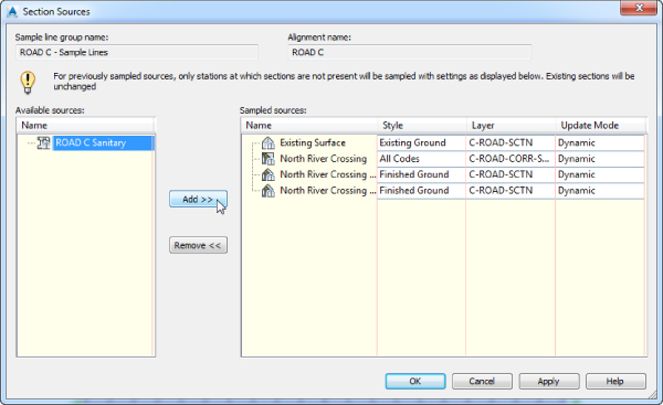
Figure 12.21 Adding sanitary pipe network to the cross-section view via Sample More Sources
The sanitary network will now appear on the right side of the dialog.
- Click OK to dismiss the Section Sources dialog.
Take a look at the sections. You should now see pipes and structures in the various section views.
Sometimes the sections views placed on the sheets might come close to overlapping the sheet border. To fix or avoid this, make sure you have well defined settings for the generation of section views sheets in your template to take into account any future data added using the Sample More Sources.
- Save the drawing for use in the next exercise.
Check your completed drawings at this stage against 1206_FinalTouches_A.dwg or 1206_FinalTouches_A_METRIC.dwg if desired.
Adding Cross-Section Labels
The best way to label cross sections that contain corridor data is to use the code set style. Using the code set style, you can control which parts of the corridor are labeled. You can learn more about creating code set styles in Chapter 18, “Label Styles.” In the meantime, you will look at how to change the active code set style on a cross-section view group.
In the following exercise, you will use the view group properties to add labels:
- Continue working in
1206_FinalTouches.dwg(1206_FinalTouches_METRIC.dwg) or open1206_FinalTouches_A.dwg(1206_FinalTouches_A_METRIC.dwg). - Select one of the section views by clicking its station label.
 From the Section View contextual tab Modify View panel, choose View Group Properties.
- On the Sections tab, locate the Style column for the corridor and click the field that currently reads All Codes.
This is the code set style that is current in the views.
- Click the field again to switch the style to Codes With Labels from the drop-down list, as shown in Figure 12.22, and click OK to dismiss the Code Set Style dialog. Click OK once more to dismiss the Section View Group Properties dialog. Press Esc to deselect the selected section view.
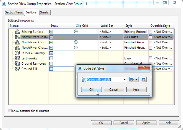
Figure 12.22 Changing the active code set style for all views in the group
You will notice that the only labels that you see are the pavement grade labels. In order to show the elevation and offsets labels, you will use a feature introduced in the current release. This feature uses labels from within the section labels part of the Settings tab in Toolspace. The advantage of using these new labels is that you can automatically stagger labels, making it easier to manage their placement in the section view.
The point labels within the code sets are considered legacy elements and are still available to display if needed. If you ever need to create the section views using the legacy code set labels for points, you can change the setting from Section Label Set to Section Code Set Style, as shown in Figure 12.23. Note that this has to be done before the creation of the cross-section views.
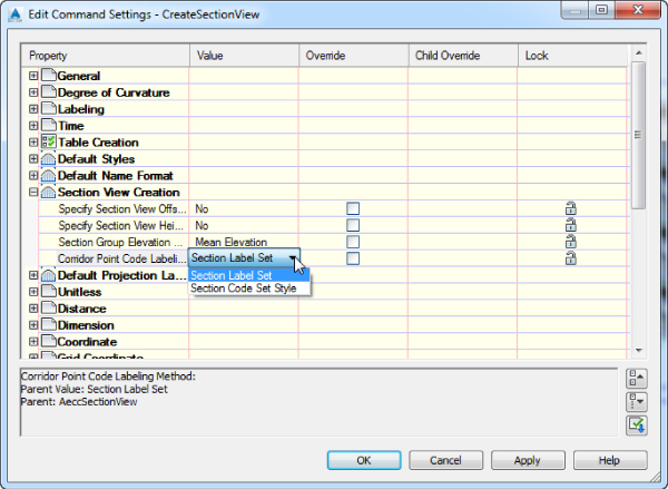
Figure 12.23 Change command settings before creating section views to maintain legacy point labels.
- Select one of the section views by clicking its station label and from the Section View contextual tab Modify View panel, choose View Group Properties.
- Click within the cell for Label Set assigned to the corridor, which is located to the left of the Code With Labels cell that you assigned previously.
- In the Select Label Set dialog, in the drop-down menu select Corridor Points. Click OK twice to apply the label set and dismiss the dialog. Press Esc to deselect the section view.
You should now have lovely little labels on all of the views, as shown in Figure 12.24. Next, you will convert one of the section views to display the legacy labels for corridor points.
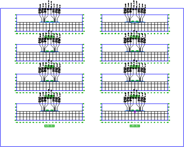
Figure 12.24 Slope, elevation, and offset labels from the code set style and corridor section labels
- At the command line type in
CORRIDORSECTIONLABELSCONV. Hit the Enter key and at theSelect section views you want to convert:prompt, pick the section view at station 10+50.00 (0+340.00 for metric users) and press the Enter key to accept the selection. - At the
Convert all corridor point labels to [Code set style labels corridor Points style labels] <Code set style labels>:prompt, press Enter once more to accept the default. - The section view will be converted to legacy mode and the code set style defined labels for points will be now displayed for the converted section view.
Check the result of you work, and then save and close the drawing.
Check your work against the file 1206_FinalTouches_FINISHED.dwg or 1206_FinalTouches_METRIC_FINISHED.dwg if time permits and you have the inclination.
Using Mass Haul Diagrams
Mass haul diagrams help designers and contractors gauge how far and how much soil needs to be moved around a site. Figure 12.25 shows the mass haul diagram for a road named Syrah Way. The free haul area is material the contractor has agreed to move at no extra charge. The fact that the mass haul line is always above 0 indicates that the project is in a net cut situation through the length of the Syrah Way alignment.
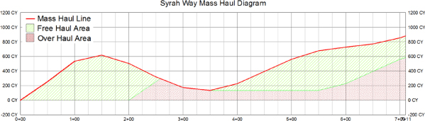
Figure 12.25 Syrah Way Mass Haul diagram (Note that the legend was added for illustration purposes only.)
Taking a Closer Look at the Mass Haul Diagram
In an ideal design situation, there is no leftover cut material and no extra material needs to be brought in. This would mean that net volume = 0. When the line appears above the zero volume point, it is showing net cut values.
As the mass haul diagram continues, it shows the cumulative effect of net cut and fill for the alignment. When the net cut and net fill converge at the zero volume, the earthwork along the alignment is balanced. When the line appears below the zero volume point, it is showing net fill values, as you can see in Figure 12.26.
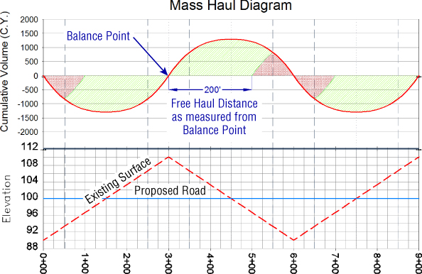
Figure 12.26 The volume, net cut, and net fill on an idealized mass haul diagram shown with profile
Here is some of the terminology you will encounter:
- Balanced The state where the cumulative cut and fill volumes are equal.
- Origin Point The beginning of the mass haul diagram, typically at station 0+00, but it can vary depending on your stationing.
- Borrow A negative value, typically at the end of the mass haul diagram, that indicates fill material that will need to be brought into the site.
- Waste A positive value, typically at the end of the mass haul diagram, that indicates cut material that will need to be hauled out of the site.
- Free Haul Earthwork that a contractor has contractually agreed to move. This typically specifies a contracted distance.
- Over Haul Earthwork that the contractor has not contractually agreed to move. This excess can be used for borrow pits or waste piles.
Create a Mass Haul Diagram
Now, let's put it all together and build a mass haul diagram in Civil 3D for Syrah Way and you'll see how easy it is:
- Open the
1207_MassHaul.dwg(1207_MassHaul_METRIC.dwg) file.Remember, you can download all the data files from this book's web page.
 From the Analyze tab Volumes And Materials panel, choose Mass Haul.
The Create Mass Haul Diagram Wizard opens.
- On the General page, complete these steps:
- Verify that you are creating a mass haul diagram for the Syrah Way alignment.
- Verify that you are using the Syrah Way - Sample Lines group.
- Leave all other options at their defaults, as shown in Figure 12.27, and click Next.
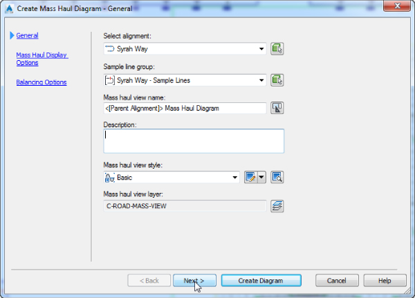
Figure 12.27 The General options of the Create Mass Haul Diagram Wizard
On the Mass Haul Display Options page, no changes are needed.
- Click Next.
- In the Balancing Options page, place a check mark next to Free Haul Distance.
- Set the distance to 200 (60 for metric users), as shown in Figure 12.28, and click Create Diagram.
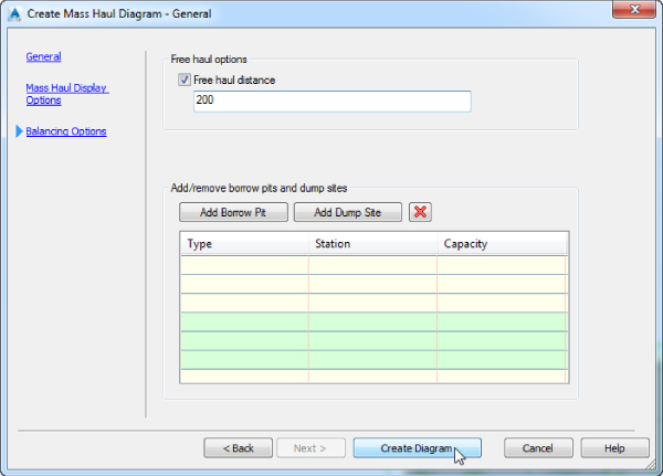
Figure 12.28 The Balancing Options page of the Create Mass Haul Diagram Wizard
- Find a clear spot on your drawing to place the mass haul diagram.
The diagram should look similar to Figure 12.25 (shown previously). Note that the legend was added for explanation purposes and is not generated by Civil 3D. We created this using AutoCAD text and hatching tools.
- Save the drawing and keep it open for the next exercise.
Check your completed drawing at this stage against 1207_MassHaul_A.dwg or 1207_MassHaul_A_METRIC.dwg if desired.
Editing a Mass Haul Diagram
When you create a mass haul diagram, you can easily modify parameters and get instant feedback on it. Follow these steps to see how:
- If you completed the previous exercise, continue working in
1207_MassHaul.dwg(1207_MassHaul_METRIC.dwg); otherwise open1207_MassHaul_A.dwg(1207_MassHaul_A_METRIC.dwg). - Select anywhere on the mass haul object or grid.
If you look at your mass haul diagram, you can see that nearly all the earthwork for Syrah Way involves net cut, which means hauling away dirt.
The Balancing options give you a chance to change or add waste and borrow pits. You will now make a few changes and observe what happens to the mass haul diagram.
 Select Mass Haul View or Mass Haul Line and from the Mass Haul View (or Mass Haul Line) contextual tab Modify panel, click the Balancing Options button.
The Mass Haul Line Properties dialog opens with the settings you used when initially generating the mass haul diagram.
- Free Haul Distance is presently set for 200 (60 for metric users). Change it to 500′ (150 m).
- Drag the dialog away from the screen to see the changes and then click Apply.
You can further tweak this amount to cut down on the net cut values by adding a dump site.
- Click the Add Dump Site button.
- Set the station to 1+31.00 (0+040.00).
- Set the capacity to 850 cubic yards (650 cubic meters).
- When your dialog resembles Figure 12.29, click OK.
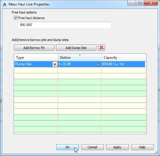
Figure 12.29 The Mass Haul Line Properties dialog: adding a dump site
The mass haul diagram will immediately update to reflect the changes. If the mass haul view does not reflect the desired layout, don't worry. Upon saving the drawing, closing it, and opening it again, the desired layout should be displayed.
- Save and close the drawing.
If you'd like to compare how you did, open the file 1207_MassHaul_FINISHED.dwg or 1207_MassHaul_METRIC_FINISHED.dwg.
For this stretch of the project, the mass haul diagram ends near zero. The changes you made also decrease the amount of overhaul in the project, potentially decreasing the earthwork cost.
The Bottom Line
- Create sample lines. Before any section views can be displayed, sections must be created from sample lines.
- Master It Open
MasterIt_1201.dwg(MasterIt_1201_METRIC.dwg) and create sample lines along the USH 10 alignment every 50 units (20 for metric users). Sample all data, and set the left and right swath widths to 50 (20 for metric users).
- Master It Open
- Create section views. Just as profiles can be shown only in profile views, sections require section views to be displayed. Section views can be plotted individually or all at once. You can break them up into groups for plotting into sheets.
- Master It In the previous exercise, you created sample lines. In that same drawing, create section views for all the sample lines. For US units, use a cross-section scale of 1″ = 20′ on an Arch D size layout sheet. For metric units, use a cross-section scale of 1:500 on an ISO A0 size sheet. For all other options, use the default settings and styles.
- Define and compute materials. Materials are required to be defined before any quantities can be displayed. You learned that materials can be defined from surfaces or from corridor shapes. Corridors must exist for shape selection, and surfaces must already be created for comparison in materials lists.
- Master It Using
MasterIt_1201.dwg(Master It_1201_METRIC.dwg), create a materials list that compares Existing Intersection with HWY 10 DATUM Surface. Use the Earthworks Quantity takeoff criteria.
- Master It Using
- Generate volume reports. Volume reports give you numbers that can be used for cost estimating on any given project. Typically, construction companies calculate their own quantities, but developers often want to know approximate volumes for budgeting purposes.
- Master It Continue using
MasterIt_1201.dwg(MasterIt_1201_METRIC.dwg). Be sure you have completed all the previous “Master It” exercises before continuing. Use the materials list created earlier to generate a volume report. Create a web browser–based report and a total volume table that can be displayed on the drawing.
- Master It Continue using