
Chapter 4
Surfaces
One of the most fundamental elements in a three-dimensional model of any design is the surface model. As you learned in the previous chapter, once survey information is gathered and points are set with elevations, you can proceed to turn some of that information into an intelligent surface model.
This chapter examines various methods of surface creation and editing. Then it moves into discussing ways to view, analyze, and label surfaces and explores how they interact with other parts of your project.
In this chapter, you will learn to:
- Create an existing ground surface using points.
- Modify and update a TIN surface.
- Prepare a slope analysis.
- Label surface contours and spot elevations.
- Import a point cloud into a drawing and create a surface model.
Understanding Surface Basics
A surface in the Autodesk® AutoCAD® Civil 3D® program is generated using the principle of triangulation. At the very simplest, a surface consists of points. The computer generates a triangular plane using a group of three points. Each triangular plane shares an edge with another, and a continuous surface is made. This methodology is referred to as a triangulated irregular network (TIN), as shown in Figure 4.1.

Figure 4.1 A triangulated irregular network, or TIN
For any given (x,y) point, there can be only one unique z value within the surface (since slope is equal to rise over run, when the run is equal to 0, the result is “undefined”). What does this mean to you? It means surfaces created by Civil 3D have several rules:
- No Thickness Modeled surfaces can be thought of as a sheet draped over a surface; they have no thickness in the vertical direction associated with them.
- No Vertical Faces Vertical faces cannot exist in a TIN because two points on the surface cannot have the same (x,y) coordinate pair. Vertical walls or curb structures must have a slight offset of at least 0.001' (0.0001 m); otherwise, they will appear flattened.
- No Caves or Tunnels The triangular planes that make up a TIN cannot overlap. If a design requires any tunnel-like structures, you will need to accomplish this with several surfaces instead.
There are four types of surfaces in Civil 3D: TIN surfaces, grid surfaces, grid volume surfaces, and TIN volume surfaces. A TIN surface is based on a set of points using Delaunay triangulation. A grid surface is based on a Digital Elevation Model (DEM) file consisting of a set of data points arranged in a regularly spaced grid configuration. DEM files can be obtained from various mapping agencies. Volume surfaces are built by measuring vertical distances between two surfaces. Volume surfaces can be created from two grid or two TIN surfaces.
Creating Surfaces
![]()
When you first create a surface in Civil 3D, you give it a name and set its style. Initially, your surface will be empty, containing no data; your next step is to add data to the surface definition.
In Prospector, you can view the contents of the surface by expanding its branch and then further expanding the Definition area, as shown in Figure 4.2.

Figure 4.2 Create a new surface (left). Expand a surface's definition to add or modify elevation data (right).
The following components can be used as part of a surface definition:
- BoundariesBoundaries are closed polylines that determine data inclusion and visibility for the surface. A boundary can be a 2D polyline, a 3D polyline, or even a feature line, but only the horizontal information will be used to generate the boundary—the elevation of the polyline is ignored. If the polyline that created the boundary is modified, the surface will become out of date.
- BreaklinesBreaklines are used to create triangulation paths, thereby preventing triangle lines that could be generated off adjacent points from crossing these paths. Breaklines are mandatory for defining flow lines, curb lines, ditch lines, pavement edges, or any linear representation of ridges or valleys. Breaklines can be defined using lines, arcs, 2D polylines, 3D polylines, survey figures, parcels, or feature lines. Similar to boundaries, if a breakline is modified, the surface will become out of date, thus requiring a rebuild. Breaklines will be discussed in more detail later in this chapter.
- Contours Polyline representations of surfaces can be used to create a Civil 3D surface. These polylines must be assigned the elevation of the contour they represent. Points will be placed along the contours to be used in the triangulation process. In addition, algorithms are run to ensure that the Civil 3D contours generated closely match the polyline contours used to define the surface. This process will be discussed in more detail later in this chapter in the section “Surfaces from Polylines.” Similar to boundaries, if the polyline contour is modified, the surface will become out of date, thus requiring a rebuild. Adding contour data will be discussed further later in this chapter.
- DEM FilesDigital Elevation Model (DEM) files are the standard format files from governmental agencies and geographic information system (GIS) systems. These files are typically large in scale but can be great for planning purposes.
- Drawing Objects These are AutoCAD objects that have an insertion point at an elevation (e.g., text, blocks, lines, AutoCAD points, 3D faces, or polyfaces) that can be used to populate a surface with elevation data. For text and blocks, the text insertion point z position is used as the elevation. Changes to these objects will not cause the surface to become out of date.
- Edits Any manipulation after the surface is completed, such as adding or removing triangles or changing the datum, will be part of the edit history. These changes can be viewed in the surface properties, where edits can be toggled on and off individually to simplify reviewing and changing. They can also be reordered since edits are applied in the order in which they are added.
- Point Files Point files work well when you're working with large data sets where the points themselves don't necessarily contain extra information. Examples include laser scanning or aerial surveys. A drawing will stay referenced to a point file. If the point file is moved or deleted, the reference in the drawing will be broken unless a surface snapshot is taken. Snapshots will be discussed later in the chapter.
- Point Groups Civil 3D point groups or survey point groups can be created to isolate a set of points used to build a surface. The surface is linked to that point group. If points are added, removed, or modified in the point group, the surface will become out of date and must be rebuilt.
- Point Survey Queries and Figure Survey Queries Point survey queries and figure survey queries perform similar tasks. A saved survey query created on the Survey tab of Toolspace can be used similarly to a point group for populating surface elevation data.
- If the query contains both points and figures, you can choose to use both types of data, only points, or only figures. Unlike a point group, data from the query can be added without the points or figures being inserted in the drawing. Prior to adding point survey queries or figure survey queries to surfaces, you must open the survey database containing those queries.
Creating a Surface with Point Groups
Usually, existing surfaces are created from data collected from topographic surveys. From that data, a set of relevant surface points can be isolated by defining a point group. This point group is a quick means of adding point data to a surface definition. Point groups are covered in Chapter 3, “Points.”
In the exercise that follows, you'll build your first basic surface with a point group:
- Open the file
0401_SurfaceFromPointGroup.dwg(0401_SurfaceFromPointGroup_METRIC.dwg), which you can download from this book's web page,www.sybex.com/go/masteringcivil3d2016. - On the Home tab of the ribbon
 Create Ground Data panel, select Surfaces Create Surface.
 - In the Create Surface dialog, shown in Figure 4.3, click in the Name field.
- Remove the default text by highlighting it and replacing it with the name Existing Surface.
- Set Style to Contours 1' and 5' (Background) or Contours 0.5 m and 2.5 m (Background) for metric users and click OK.
- In Prospector, expand the Surfaces branch. You should now see your new surface in the listing.
- Expand Existing Surface and then expand Definition by clicking the tiny plus sign to the left of the listing in Prospector.
- Right-click Point Groups and select Add.
- In the Point Groups dialog, highlight TOPO Shots and click OK. You should now see contours for your surface.
- Save your drawing at the conclusion of the exercise. Compare your work with
0401_SurfaceFromPointGroup_FINISHED.dwgor0401_SurfaceFromPointGroup_METRIC_FINISHED.dwgif desired.

Figure 4.3 Creating your first new TIN surface
Adding Breaklines
Breaklines change the triangulation of a surface by forcing triangle edges to follow along the segments of the breakline. Breaklines represent linear features where a change in the slope of a surface occurs. Examples of such features would be ridges, streams, ditches, curbs, and retaining walls, just to name a few.
There are several methods for adding breaklines to a surface. On the Prospector tab of Toolspace, you can select the Breakline branch of the surface definition, right-click, and select Add. Additionally, you can easily add survey figures by going to the Survey tab of Toolspace, right-clicking the Figures branch, and selecting Create Breaklines. When feature lines are selected, an Add To Surface As Breakline option is displayed in the contextual tab.
Breakline Types
No matter which method you use to add breaklines to a surface's definition, you will need to configure the type of breakline that it is. The breakline types are as follows:
- Standard Standard breaklines can be 2D or 3D polylines, arcs, lines, splines, feature lines, figures, or parcels. These entities have the actual elevations for the surface assigned at their vertices. The vertex elevations become surface points, TIN lines are drawn along the breakline, and then the remaining triangulation is calculated. Standard breaklines represent both the horizontal and vertical locations of linear features of a surface.
- Proximity Proximity breaklines represent horizontal location only. In fact, if the entity used to define the proximity breakline is 3D, the vertex elevation will be ignored. The elevation of each vertex is determined from a nearby surface point already added to the surface.
- Wall Wall breaklines can be used to define near-vertical drops such as retaining walls or curb lines. You would define a wall breakline much the same as you would define a standard breakline. After selecting the feature, you would define a horizontal offset side and then an elevation difference at each vertex or for the entire length of the feature.
- From FileThe From File option is needed only if you have an FLT text file containing breakline data. This file type is usually the result of output from another program and contains XYZ data on each vertex for the lines described in the file. Once the FLT file has been imported, the effect on the surface is identical to a standard breakline. File Link options can be dynamically linked to the file, or the link can be broken so the surface will no longer be dependent on the file.
- Non-destructive Non-destructive breaklines neither change elevation nor change grades of the surface model. Non-destructive breaklines simply control the horizontal orientation of triangle lines. You may find yourself needing a non-destructive breakline in anticipation of cleaning up triangle data, as discussed later in this chapter, in the section “Manual Surface Edits.”
By far, standard is the most frequently used type of breakline, followed by proximity and wall breaklines.
Weeding Factors
Turning on Weeding Factors in the Add Breaklines dialog allows you to omit extraneous data from your surface. You will want to consider weeding when your breaklines contain a lot of vertices very close together. Each vertex is added to your surface as a point, so when you weed, your aim is to exclude extraneous point data. This not only reduces the size of your surface but helps to eliminate the formation of skinny triangles, which can produce saw-toothed contours.
Weeding requires that a distance and angle be entered in the Add Breaklines dialog. With these settings, the program will examine each vertex as follows:
- It measures the length of the segment leading into the vertex.
- It measures the length of the segment leaving the vertex.
- If the sum of both lengths is less than the entered distance value, it checks the delta angle.
- If the delta angle is less than the entered angle value, it omits the vertex.
Supplementing Factors
Turning on Supplementing Factors in the Add Breaklines dialog enables you to add additional surface points along your breaklines. Doing this helps to eliminate the generation of long triangle lines. It also allows you to define breaklines more precisely along curves.
The Distance setting works like the AutoCAD measure command. When breaklines are added to a surface, Civil 3D will add additional vertices based on this increment value.
The Mid-ordinate Distance setting is applied to arc segments in your breaklines. If this setting were absent, the program would create a single breakline segment from the PC to the PT of the arc. With this setting in place, the program creates shorter segments along the arc. With each segment considered to be tiny chords, the Mid-ordinate Distance value is the resulting measurement from the midpoint of each chord to the midpoint of each segmented arc.
In this example, you'll add some breaklines that describe road and ditch features:
- Open the
0402_SurfaceFromBreaklines.dwgfile or the0402_SurfaceFromBreaklines_METRIC.dwgfile.This drawing is similar to the drawing used in the first exercise. It contains a surface created with a point group. It also contains 3D survey figures. Without the survey database, you'll have to add the figures conventionally, meaning through the Breakline branch of the surface.
- Inspect the drawing by panning and zooming along the linework.
Notice that the TIN lines are not drawn along the figures representing the edge of pavement, centerline of roads, flowline of ditches, and top of banks.
- Select and then right-click one of the brown figures representing the top of bank, and choose the Select Similar option.
The tooltip will indicate a figure prefix style of TB.
All the brown figures representing the tops of banks are now highlighted.
- In Prospector, expand the Surfaces Existing Surface Definition branches.
- Right-click Breaklines and select the Add option.
The Add Breaklines dialog appears.
- Enter the description Top of Bank and leave all other settings at their default, as shown in Figure 4.4.
- Click OK to accept the settings and close the dialog.
You can dismiss Panorama if it appears.
- Repeat steps 3–7 for figures DL (Flowline of Ditch), BB (Bottom of Bank), CL (Centerline of Road), and EP (Edge of Pavement).
- Zoom extents and notice that the TIN lines are now running along the survey figures now acting as breaklines.

Figure 4.4 Entering a description in the Add Breaklines dialog
As shown in Figure 4.5, by adding the breaklines, you force the TIN lines to align with them, thus cleaning up the contours and making them follow the ridgelines of the road centerline, gutter lines, and shoulders as well as the changes in grade around the small detention area.

Figure 4.5 Existing surface with contours displayed before breaklines are added (left) and after (right)
When this exercise is complete, you can close the drawing. A completed version of this drawing is available from the book's web page with the filename 0402_SurfaceFromBreaklines_FINISHED.dwg or 0402_SurfaceFromBreaklines_METRIC_FINISHED.dwg.
Adding Boundaries
Use boundaries when you want to restrict the area where triangles are being generated. Many object types can be used as surface boundaries, such as survey figures, feature lines, 2D polylines, and 3D polylines. Whatever type of line you choose as your boundary, it must be closed and cannot cross itself (i.e., no “loop-the-loops”). Elevations of the boundaries are ignored. There are four types of surface boundaries:
- Outer Outer boundaries are used to conceal surface components (triangles, contours, or points) occurring outside the boundary extents.
- Hide Hide boundaries are used to conceal surface components inside the boundary extents. For example, consider a hide boundary to hide any interpolation occurring inside a building perimeter.
- Show Show boundaries are used to reveal surface components inside a hide boundary. If a hide boundary was used around a building perimeter, a show boundary can be applied to reveal contours in the building's courtyard for landscape purposes. Show boundaries can also be used to show surface areas outside an outer boundary.
- Data Clip A data clip is a type of boundary drawn around the extents of a site. It is used to prevent surface calculations from occurring beyond its extents. The data clip boundary should be the first component added to the surface definition. For example, if a DEM file representing the surface of an entire county will be used to create a surface, a data clip boundary can be applied first to exclude the grid information outside the construction site. Using a data clip boundary will result in smaller surfaces (fewer surface points), which will impact your file size.
The addition of every boundary is considered a separate part of the building operations. This means that the order in which the boundaries are applied controls their final appearance. For example, a show boundary listed before a hide boundary created in the same area will be overridden by that hide operation.
One way to start defining more accurate boundaries is to first extract the boundary defining the extents of the surface to a polyline and then edit the polyline to the optimum shape. The Extract Objects From Surface utility allows you to re-create any displayed surface element (contours, border, and the like) as an independent AutoCAD entity. It is important to note that only the objects that are currently visible in the surface style can be extracted. In this exercise, you'll extract the existing surface boundary as a starting point for creating a more refined boundary that will limit triangulation:
- Open the
0403_SurfaceBoundary.dwgor0403_SurfaceBoundary_METRIC.dwgfile. - Select the surface.
- From the TIN Surface contextual tab Surface Tools panel, choose Extract From Surface Extract Objects to open the Extract Objects From Surface dialog.

- Leave the Border object selected and deselect the Major Contour, Minor Contour, and Points options, as shown in Figure 4.6.

Figure 4.6 Extracting the border from the surface object
- Click OK to finish the process. Press Esc to deselect the surface.
A 3D polyline has been created from the surface border.
- Pick the border 3D polyline.
This polyline will form the basis for your outer surface boundary. By extracting the border polyline from the existing surface, you save a lot of time playing connect the dots along the points that are valid. Next, you'll add this polyline into the surface as a boundary.
- In Prospector, expand the Surfaces Existing Surface Definition branches.
- Right-click Boundaries and select the Add option.
The Add Boundaries dialog opens (Figure 4.7).

Figure 4.7 Add Boundaries dialog
- Enter the name Outer, leave Type set to Outer, and keep the check mark next to the Non-destructive Breakline option; then click OK.
- Pick the 3D polyline border that you previously extracted.
- Working your way around the site clockwise, grip-edit the polyline you created in step 6 to exclude some of the area at the northwest area of the site around the ditch where there are no points. Use the Add Vertex option from the grip menu, as shown in Figure 4.8.

Figure 4.8 Using the grips to adjust the border
Note that this process does not require you to use object snaps. This boundary only needs to be approximate. You will see the surface dynamically update with each grip edit since the surface is set to Rebuild Automatic.
- If time permits, edit the entire boundary.
On a large site, you can see that this is a time-consuming process but worth the effort to clean up the site nicely (Figure 4.9). Thankfully, there are other methods you can use to clean up the surface border; we will discuss these methods in later exercises.

Figure 4.9 A non-destructive outer boundary in action
- Save the drawing and keep it open for the next portion of the exercise.
Notice in some areas along the outer boundary how the edge of the triangulation includes points shown as a square with a + symbol; these are the additional points created along the boundary line where it intersects with the triangles it crosses. The points you attempted to exclude from the surface are still being included in the calculation of elevations for this point; they are just excluded from the display and calculations. This isn't the result you were after, so let's fix it now.
- In Prospector, expand the Surfaces Existing Surface Definition branches and select Boundaries.
A listing of the boundaries appears in the preview area of Toolspace.
- Right-click the boundary you just created and select the Delete option.
- Click OK in the warning dialog that tells you the selected definition items will be permanently removed from the surface.
You can dismiss Panorama if it appears.
- In Prospector, right-click Boundaries and select the Add option again.
The Add Boundaries dialog appears.
- Enter the name Outer, leave Type set to Outer, and leave the check box unchecked next to the Non-destructive Breakline option; then click OK.
- Pick the revised 3D polyline again.
Notice that no triangles intersect your boundary now where it does not connect points, as shown in Figure 4.10.

Figure 4.10 A destructive outer boundary in action

Figure 4.11 Adding buildings as non-destructive, hide boundaries
Next, you will add a hide boundary to the surface.
- In Prospector, right-click Boundaries and select the Add option again.
- Name the boundary Buildings and change Type to Hide. Make sure that Non-destructive Breakline is checked, as shown in Figure 4.11, and click OK.
- Select the outer outline of the cyan building in the northwest portion of the site. Press Enter.
You should now have a void in your surface where the building exists.
- Right-click Boundaries and select the Add option one last time.
- Name the boundary Courtyard, set the type to Show, and verify that Non-destructive Breakline is checked.
- Click OK; then click the closed polyline inside the building outline and press Enter.
You should now see an island of surface data inside the previously hidden location.
When this exercise is complete, you can close the drawing. A finished copy of this drawing is available from the book's web page with the filename 0403_SurfaceBoundary_FINISHED.dwg or 0403_SurfaceBoundary_METRIC_FINISHED.dwg.
Additional Surface Creation Methods
Many forms of data can be processed by Civil 3D to create a surface. The data types discussed in the following sections are common when working with organizations that are not using Civil 3D.
File types like TIN and LandXML are often best for moving data from other civil design software programs into Civil 3D. DEM files can be used to create surfaces for preliminary drainage analysis.
- TIN Files A TIN file represents a surface that was generated by AutoCAD Land Desktop. The corresponding PNT file from the Land Desktop surface folder must be present in the same folder as well. These files contain the baseline TIN information from the original surface and can be used to regenerate it easily.
- LandXML Files LandXML files can be exported from most land development software applications for use in another land development software application. LandXML has become a common means of migrating data in the land development industry. LandXML files contain the point elevations along with the associated 3D face definitions resulting from the creation and surface edits performed in the originating software application.
- Digital Elevation Models Digital Elevation Model files are used by the U.S. Department of the Interior's United States Geological Survey (USGS) and are commonly produced by government organizations for their GIS systems. The DEM format can be read directly by Civil 3D, but the USGS typically distributes the data in a complex format called Spatial Data Transfer Standard (SDTS). The files can be converted using a freely available program named
sdts2dem. This DOS-based program converts the files from the SDTS format to the DEM format you need. Once you are in possession of a DEM file, creating a surface from it is relatively simple.
Surface from LandXML Files
Oftentimes, the engineering and survey tasks for a land development project are performed by separate companies. If you are tasked with the engineering design and are receiving a DWG file representing the existing site with contours from another firm, you should ask for a LandXML export of the existing surface. It is much more precise than using the contours to build your existing surface. It will also save time as compared with building the surface from scratch with points and breaklines.
- Create a new drawing using the
_AutoCAD Civil 3D (Imperial) NCStemplate. Metric users should use the_AutoCAD Civil 3D (Metric) NCStemplate. - Switch to the Settings tab of Toolspace, right-click the drawing name, and select Edit Drawing Settings.
The Drawing Settings dialog appears.
- Imperial users should set the zone category to USA, North Carolina, and set the coordinate system to NAD83 North Carolina State Planes, US Foot (NC83F) via the Units And Zone tab of the Drawing Settings dialog. Metric users should set the zone category to USA, North Carolina, and set the coordinate system to NAD83 North Carolina State Planes, Meter (NC83).
- Click OK.
- From the Insert tab Import panel, choose LandXML.
The Import LandXML dialog appears.
- Select
0404_SurfaceFromFile.XMLand click Open to continue.The Import LandXML dialog changes, as shown in Figure 4.12.

Figure 4.12 Understanding the Import LandXML dialog
- In the Import LandXML dialog, expand the Surfaces collection.
Notice the check boxes. A LandXML file can contain many forms of design data such as alignments, profiles, parcels, points, and pipe networks as well as surfaces. If you receive a file with multiple forms of design data, here in this dialog is where you would uncheck what you do not want to import into the immediate drawing. It isn't possible to uncheck Units, Project Name, or Application Description. These lines are in there for informational purposes only, giving a history of the file: originating units, originating drawing name, originating application. In this example, the originating application was Civil 3D. Sometimes firms make it a policy of not sharing their object data (in this case, the existing surface) when performing file exchanges. This is so they can retain ownership of the model and keep their styles in house. We'll discuss more about styles in Chapter 19.
- Click Edit LandXML Settings.
The LandXML Settings dialog appears.
- Expand the Surface Import Settings collection and configure these settings to match Figure 4.13.

Figure 4.13 Configuring Surface Import Settings
- Click OK to continue and OK again to close the Import LandXML dialog.
After the surface imports, Civil 3D will zoom extents.
- In Prospector, expand the Surfaces Existing From LandXML Definition collection and click Definition.
Notice in the list view that no data is being used in the surface definition. The definition of this surface is coming directly from the LandXML file. As a matter of fact, if this LandXML file were moved or deleted, the surface definition would be lost if it weren't for the automatic creation of a snapshot.
- Right-click the Existing From LandXML Surface and click Surface Properties.
- On the Definition tab, notice the Data Operations list on the bottom half of the dialog.
The first item on the list is the Import XML File operation. Notice the Browse button next to the path to the file. This button can be used to redefine the path to the LandXML file if the location must change or the file gets renamed. The next line contains the Create Snapshot operation, which preserves the surface definition in case the XML file is lost. Either line can be deleted from the surface definition. Since a snapshot ignores any previous surface operations, if a new XML file is sent to you containing an updated surface definition, you would need to delete and then re-create the snapshot based on the new definition.

- Click OK to close the Surface Properties dialog.
A completed version of this drawing is available from the book's web page (0404_SurfaceFromFile_FINISHED.dwg or 0404_SurfaceFromFile_METRIC_FINISHED.dwg).
Surface from DEM Files
In the following exercise, you will be creating a surface from a DEM file:
- Start a new drawing from the
_AutoCAD Civil 3D (Imperial) NCStemplate that ships with Civil 3D. Metric users should use the_AutoCAD Civil 3D (Metric) NCStemplate. - Switch to the Settings tab of Toolspace, right-click the drawing name, and select Edit Drawing Settings.
The Drawing Settings dialog appears.
- Imperial users should set the zone category to USA, North Carolina, and set the coordinate system to NAD83 North Carolina State Planes, US Foot (NC83F) via the Units And Zone tab of the Drawing Settings dialog. Metric users should set the zone category to USA, North Carolina, and set the coordinate system to NAD83 North Carolina State Planes, Meter (NC83).
- Click OK.
The coordinate system of the DEM file that you will import will be adjusted to the coordinate system of the drawing.
- From the Home tab Create Ground Data panel, choose Surfaces Create Surface.
The Create Surface dialog appears. If a coordinate system transformation wasn't necessary, Create Surface From DEM would be a quicker method for creating this surface. However, Create Surface From DEM produces a grid surface, which cannot be adjusted.
- Accept the options in the dialog, and click OK to create the surface.
This surface is added as Surface1 to the Surfaces collection in Prospector.
- In Prospector, expand the Surfaces Surface1 Definition branches.
- Right-click DEM Files and select the Add option (see Figure 4.14).

Figure 4.14 Adding DEM data to a surface
The Add DEM File dialog appears.
- Use the button to the right of the DEM File Name area to navigate to the
0405_Camden_NC.DEMfile and click Open.
Remember, you can download all data and drawing files for this book from
www.sybex.com/go/masteringcivil3d2016. The DEM file information will populate in the Add DEM File dialog, showing that the DEM file you are using is UTM Zone 18, NAD27 Datum, Meters. - In the Add DEM File dialog, click in the Value column next to CS Code to display the ellipsis button; click that button to display the Select Coordinate Zone dialog.
- Both Imperial and metric users, set the coordinate system code (CS code) to match the DEM file by selecting UTM With NAD27 Datum, Zone 18, Meter; Central Meridian 75d W (UTM27-18), as shown in Figure 4.15, and click OK.

Figure 4.15 Setting the
0405_Camden_NC.DEMcoordinate zoneNote that you can find the coordinate system information for this DEM by reviewing the DEM file information section of the Add DEM File dialog.
This information is necessary to properly translate the DEM's coordinate system to the drawing's coordinate system.
The Add DEM File dialog should now match the one shown in Figure 4.16.

Figure 4.16 Setting the
0405_Camden_NC.DEMfile properties - Click OK in the Add DEM File dialog.
You may receive a message regarding the level of detail, which is discussed later in this chapter. If a Level Of Detail dialog appears, click the Keep The Current Display Mode option.
- In Prospector, right-click Surface1 and select Zoom To to bring the surface into view.
- Select the surface. From the Surface contextual tab of the ribbon Modify panel, click the Surface Properties icon.
The Surface Properties dialog appears. Earlier, in the Create Surface dialog, you allowed the default surface name to be used, which created the name of Surface1. Since the default name does not provide much information, you will now revise the default name to something that offers more information to the user.
- On the Information tab, change the Name field entry to Camden Point NC.
- Change the Surface Style drop-down list to Contours And Triangles and then click OK to accept the settings in the Surface Properties dialog.
Once you have the DEM data imported, you can pause over any portion of the surface and see that feedback showing the surface elevation is provided through a tooltip. This surface can be used for preliminary analysis but isn't accurate enough for construction purposes.
The main drawback to DEM data is the sheer bulk of the surface size and point count. The 0405_Camden_NC.DEM file you just imported contains 173,185 points and covers more than 60 square miles. This much data can be overwhelming, and it covers an area much larger than the typical site. If you try zooming in and out on the surface, you may notice performance lag. To ease the processing and activate the Level Of Detail display, do the following:
- Switch to the View tab on the ribbon.
- Expand the bottom of the Views panel.
- Select Level Of Detail. A Level Of Detail Display warning message may appear. If so, click Close.
![]()
After these steps are complete, you will notice that a new icon appears in the upper-left corner of your model space, showing you that Level Of Detail is activated. To turn off Level Of Detail, follow the same steps.
Turning on the Level Of Detail display does not change the data in the surface but simply changes what is viewable at the different zoom levels. Figure 4.17 shows the same area of the surface before turning on Level Of Detail (left) and after (right). The left version of the surface appears shaded because that is how dense the triangles are. You'll look at some data reduction methods later in this chapter.

Figure 4.17 DEM surface: shown without Level Of Detail (left), zoomed out with Level Of Detail (right)
With Level Of Detail turned on, save your drawing at the conclusion of the exercise. Compare your work with 0405_SurfaceFromDEM_FINISHED.dwg or 0405_SurfaceFromDEM_METRIC_FINISHED.dwg if desired.
Surface from GIS Data
Whether the source is internal or from an outside firm, elevation data from geographic information systems is becoming increasingly common. Civil 3D understands GIS and can work with the data given. In this section, we'll show you how to import GIS data pertaining to surfaces:
- Start a new drawing by using the
_AutoCAD Civil 3D (Imperial) NCStemplate and set the coordinate system to NAD83 Virginia State Planes, North Zone, US Foot (VA83-NF). Metric users should use the_AutoCAD Civil 3D (Metric) NCStemplate and set the coordinate system to NAD83, Virginia State Planes, North Zone, Meter (VA83-N). - From the Home tab Create Ground Data panel, choose Surfaces Create Surface From GIS Data.
The Create Surface From GIS Data – Object Options page appears.
- Set Name to GIS Data, change Description to Import from GIS Data, and set the style to Contours 5' and 25' (Background) or Contours 2 m and 10 m (Background) for metric users, as shown in Figure 4.18; then click the Next button.

Figure 4.18 The Create Surface From GIS Data – Object Options page
The Create Surface From GIS Data – Connect To Data page appears.
- You are importing a SHP file, so change Data Source Type to SHP.
- Click the ellipsis next to SHP Path. Locate the
0406_Contours.shpfile (which you'll find atwww.sybex.com/go/masteringcivil3d2016). Then click Open.The path is now populated with the location of the SHP file, as shown in Figure 4.19.

Figure 4.19 The Create Surface From GIS Data – Connect To Data page
- Click the Login button.
You won't need a username or password to log in.
The Create Surface From GIS Data – Schema And Coordinates page now appears (Figure 4.20).

Figure 4.20 The Create Surface From GIS Data – Schema And Coordinates page
You will notice that the name of the file appears as well as the coordinate system in which the SHP was created. If you are an Imperial user, the NAD83 Virginia State Planes, North Zone, US Foot system matches what you set the drawing up with. For metric users, the coordinate system of the SHP file is different from the drawing coordinate system.
- Verify that the 0406_Contours check box is checked under Feature Class and click Next.
- On the Create Surface From GIS Data – Geospatial Query page, look at the settings for future reference, but do not make any changes (Figure 4.21). Click Next.

Figure 4.21 The Create Surface From GIS Data – Geospatial Query page
- On the Create Surface From GIS Data – Data Mapping page, click the drop-down list next to FLABEL in the GIS Field column and select Elevation, as shown in Figure 4.22.

Figure 4.22 The Create Surface From GIS Data – Data Mapping page
Many dialogs throughout the software use tables such as those shown on this page for you to input data. If at any time the column is not wide enough for you to view all of the contents, you may modify the column width by clicking between the column headings.
At the bottom of the Create Surface From GIS Data – Data Mapping page you will notice a File Name field as well as Save and Open icons. That means you can save the current data mapping information that you've set for future use.
- Click the Finish button.
- Dismiss Panorama and zoom extents to see the surface based on the SHP file (Figure 4.23). If the Level Of Detail Display setting is still on from the previous exercise, turn it off (View tab Views panel expanded Level Of Detail).

Figure 4.23 The finished imported GIS contours
When this exercise is complete, you can close the drawing. A finished copy of this drawing is available from the book's web page with the filename 0406_SurfaceFromGIS_FINISHED.dwg or 0406_SurfaceFromGIS_METRIC_FINISHED.dwg.
This is just another avenue for getting data from other sources into Civil 3D.
Surfaces from Polylines
The quality of the data you receive if you are working with contours varies greatly. The contour interval and smoothing factors will affect the result when imported to Civil 3D. The resulting surface may not accurately reflect the original survey data. This is because elevation information is provided along the contour lines but not in between the contour lines, causing the interpolation between the contours to lack accuracy. Civil 3D includes a series of surface algorithms that work well at matching the resulting surface to the original contour data by providing additional derived data points. You'll look at those surface edits in this series of exercises:
- Open the
0407_SurfaceFromPolylines.dwgfile (or the0407_SurfaceFromPolylines_METRIC.dwgfile).Note that the contours in this file are composed of polylines with elevation values.
- In Prospector, right-click the Surfaces branch and select the Create Surface option.
The Create Surface dialog appears.
- Leave the Type field set to TIN Surface, but change the Name value to EG-Polylines.
- Change Description to Surface From Polylines.
- Click in the Value column next to Style to display the ellipsis button; once it's visible, click the ellipsis button to display the Select Surface Style dialog.
- From the drop-down list, select Contours 5' And 25' (Background) or Contours 2m And 10m (Background) for metric users; click OK to close the Select Surface Style dialog.
- Click OK to close the Create Surface dialog.
- In Prospector, expand the Surfaces EG-Polylines Definition branches.
- Right-click Contours and select the Add option.
The Add Contour Data dialog appears.
- Set Description to Polylines. Under Weeding Factors, set:
- Distance to 15 (or 5 for metric users)
- Angle to 4 degrees.
Under Supplementing Factors, set:
- Distance to 100 (or 30 for metric users)
- Mid-Ordinate Distance to 1 (or 0.3 for metric users).
- Verify that no check boxes are checked, as shown in Figure 4.24, and click OK.

Figure 4.24 The Add Contour Data dialog
In this example it is okay to leave all the Minimize Flat Areas By options unchecked. You will return to the Minimize Flat Areas By options in a bit.
- At the
Select contours:prompt, enter ALL ↲ to select all the entities in the drawing and press ↲ again to end the command.You can dismiss Panorama if it appears by clicking the green check mark. Save the drawing and keep it open for the next portion of the exercise.
The contour data has some tight curves and flat spots where the basic contouring algorithms simply fail. Zoom into any portion of the site, and you can see these areas by looking for the blue and cyan original contours not matching the new Civil 3D–generated contour, as shown in Figure 4.25.

Figure 4.25 Contour surface without minimizing flat areas

Figure 4.26 Contour surface with minimizing flat areas

Figure 4.27 Surface data points and derived data points
You'll fix that now.
- In Prospector, expand the Definition branch of the EG-Polylines surface if it's not already open from the previous exercise and right-click Edits.
- Select the Minimize Flat Areas option to open the Minimize Flat Areas dialog.
Note that the dialog has the same options found in that portion of your original Add Contour Data dialog.
- Click OK to accept the defaults.
- Save the drawing and keep it open for the next portion of the exercise.
Now the contours displayed more closely match the original contour information, as shown in Figure 4.26. There might be a few instances where gaps exist between old and new contour lines, but in a cursory analysis, none was off by more than 0.4' in the horizontal direction—not bad when you're dealing with almost a square mile of contour information.
- Zoom into an area with a dense contour spacing and select the surface to make the contextual tab associated with the TIN Surface: EG-Polylines appear.
- From the TIN Surface contextual tab Modify panel, choose the Surface Properties icon to display the Surface Properties dialog.
- On the Information tab, set Surface Style to Contours And Points, and click OK to see a drawing similar to Figure 4.27. Press the Esc key to deselect the surface.
In Figure 4.27, you're seeing the points the TIN is derived from, with some styling applied to help you understand the creation source of the points. Although you can't see the colors in the printed figure, on the screen the points are shown in color to help you differentiate them:
- Each point shown as a red + symbol is a point picked up from the contour data itself.
- The magenta points shown with a circle symbol circumscribed over a + symbol are all added data on the basis of the Minimize Flat Areas edits.
These points make it possible for the Civil 3D surface to match almost exactly the input contour data.
At this time, the original polylines are still present in the drawing, and you may find yourself tempted to delete them. Before doing so, you will want to change the surface property Copy Deleted Dependent Objects, as discussed in the section “Surface Build Options” later in this chapter.
When this exercise is complete, you can close the drawing. A completed version of this drawing is available from the book's web page with the filename 0407_SurfaceFromPolylines_FINISHED.dwg or 0407_SurfaceFromPolylines_METRIC_FINISHED.dwg.
Now that you have learned how to add several types of data to a surface definition, you will need to fine-tune your surface models for better accuracy.
Refining and Editing Surfaces
![]()
Once a basic surface is built, and in some cases even before it is built, you can do some cleanup and modification to the TIN construction that make it much more usable and realistic. Some of these edits include limiting the input data, tweaking the triangulation, adding breakline information, and hiding areas from view. In the following sections, you'll explore a number of ways of refining surfaces to end up with the best possible model from which to build.
Surface Properties
The most basic steps you can perform in making a better model are right in the Surface Properties dialog. The surface object contains information about the build and edit operations, along with some values used in surface calculations.
Surface Build Options
There are two main places you can set surface build options:
- Settings Tab The first location is on the Settings tab of Toolspace under Surfaces Commands Create Surface. If you right-click Create Surface, you will find an option to edit command settings. You can set these at the beginning of a project to automatically set the options for all surfaces as they are created. It is a great idea to configure the command settings in your template so your preferred triangulation defaults will be set on all projects.
- Surface Properties The second place you will see the build options for a surface is in Surface Properties on the Definition tab. Changing the settings under Surface Properties will affect only the individual surface you are working with.
The basic options are listed here:
- Copy Deleted Dependent Objects When you select Yes and an object (such as a surface boundary or breakline) that is part of the surface definition is deleted, the information derived from that object is copied into the surface definition. If this option is set to No for the surface, when elevation source objects (such as polylines added as contours) are deleted, they will be removed from the surface definition when the surface is rebuilt.
- Exclude Elevations Less Than Setting Exclude Elevations Less Than to Yes allows you to set a surface's lowest valid elevation in the Elevation < field. Note that Elevation < is a “less than” operation, not “less than or equal to,” so to rectify the problem caused by items at 0, you will need to set this to 1, for example.
- Exclude Elevations Greater Than Setting this to Yes will allow you to set the Elevation > field. This option allows you to set a highest valid elevation value.
- Use Maximum Angle Setting this option to Yes will allow you to set a value for Maximum Angle Between Adjacent TIN Lines. This setting will omit long “sliver” triangles that typically get generated along the exterior of the TIN.
- Use Maximum Triangle Length Setting this option to Yes will allow you to set a value for Maximum Triangle Length. If a triangle leg is excessively long, it is often an indicator that valid elevation data for triangulation is sparse, as often occurs near the edges of a site. If you are using this option to minimize long triangle lines, double-check your TIN to make sure the length you specified isn't creating interior holes.
- Convert Proximity Breaklines To Standard Toggling this option to Yes will create standard breaklines out of the entities used as proximity breaklines. The surface will no longer be dependent on the proximity entities. The standard breakline will be created internal to the surface but can be drawn by right-clicking the breakline in the surface definition and selecting Insert Into Drawing.
- Allow Crossing Breaklines Setting this option to Yes allows you to set the Elevation To Use option. These options specify what Civil 3D should do if two breaklines in a surface definition intersect in the X,Y plane with different elevations at the intersection. Leaving this option set to No will cause the surface to totally throw out both offending breaklines.
In this exercise, you'll go through a couple of the basic surface-building controls that are available. You'll use them one at a time in order to observe their effects on the final surface display.
- Open the
0408_SurfaceProperties.dwgfile (or the0408_SurfaceProperties_METRIC.dwgfile). - Locate the portion of the surface that contains poor elevation data inside the magenta circle. Use your mouse to pan and zoom in the drawing.
You will know you have found the correct location when you zoom into the portion of the surface that resembles Figure 4.28. This blob is a batch of densely packed contours where the surface is incorrectly picking up elevations at zero.

Figure 4.28 EG surface showing a batch of densely packed contours, indicating bad elevations
- Select the surface by clicking any part of it in the graphic.
- From the TIN Surface: EG contextual tab, click the Surface Properties icon.
The Surface Properties dialog appears.
- Select the Definition tab.
- Under Definition Options at the top of the dialog (Figure 4.29), expand the Build branch by clicking the + symbol.

Figure 4.29 Surface Properties Definition Options
- Verify that the Exclude Elevations Less Than value is Yes.
- Set the value to 200 (60 for metric users) and click OK to accept the settings in the dialog.
A warning message will appear. Civil 3D is warning you that your surface definition has changed.
- Click Rebuild The Surface to rebuild the surface.
- You may see a message appear in Panorama indicating that three points were ignored because they are below the given limit. If this is the case, close the Panorama window by clicking the green check mark.
- Zoom extents to view the full surface by double-clicking your middle mouse wheel.
When this step is complete, the surface will look similar to Figure 4.30. Save the drawing and keep it open for the next portion of the exercise.

Figure 4.30 EG surface after ignoring low elevations
Although this surface is improving, there are still large areas being contoured that shouldn't be. By changing the style to review the surface, you can see where you still have some issues.
- Open the Surface Properties dialog again and switch to the Information tab.
- Change the Surface Style field to Contours And Triangles.
- Click Apply. Doing so makes the changes without exiting the dialog.
- Drag the dialog to the side so you can see the site.
On the outer edges of the site, you can see some long triangles formed in areas where there was no survey taken but the surface decided to connect the triangles anyway (Figure 4.31, left).

Figure 4.31 EG surface before Use Maximum Triangle Length was applied (left) and after (right). Note that the Level Of Detail display option is on in these figures.
- In the Surface Properties dialog, switch to the Definition tab.
- Expand the Build category by clicking the + symbol.
- Set the Use Maximum Triangle Length value to Yes.
- In the Maximum Triangle Length value field, enter 300 (or for metric, 70).
- Click OK to apply the settings and close the dialog.
- Click Rebuild The Surface to update and dismiss the warning message to see the revised surface (Figure 4.31, right).
When this exercise is complete, you can close the drawing. A completed version of this drawing is available from the book's web page with the filename 0408_SurfaceProperties_FINISHED.dwg or 0408_SurfaceProperties_METRIC_FINISHED.dwg.
Manual Surface Edits
Manual edits allow further surface refinement by changing the surface at its core—the triangles. A number of manual edits can be performed on a surface. These edit options become part of the definition of the surface and include the following:
- Add Line Connects two points where a triangle did not exist before. This option essentially adds a breakline to the surface, so adding a breakline would generally be a better solution. This option is not available on grid surfaces.
- Delete Line Removes the connection between two points. In addition to using outer boundaries, this option is used frequently to clean up the edge of a surface or to remove internal data where a surface should have no triangulation at all. This can be an area such as a building pad or water surface, although hide boundaries are recommended in these scenarios.
- Swap Edge Changes the direction of the triangulation methodology. For any four points, there are two solutions to the internal triangulation, and the Swap Edge option alternates from one solution to the other. The necessity of numerous swap edge operations can be limited by the use of appropriate breaklines. This option is not available on grid surfaces.
- Add Point Allows for the manual addition of surface data. This function is often used to add a peak to a digitized set of contours that might have a flat spot at the top of a hill.
- Delete Point Allows for the manual removal of a data point from the surface definition. Generally, it's better to fix the source of the bad data, but this option can be a fix if the original data is not editable (in the case of a LandXML file, for example).
- Modify Point Allows for changing the elevation of a surface point. Only the TIN point is modified, not the original data input.
- Move Point Is limited to horizontal movement. Like Modify Point, only the TIN point is modified, not the original data input. This option is not available on grid surfaces.
- Minimize Flat Areas Performs the edits you saw earlier in this chapter to add supplemental information to the TIN and to create a more accurate surface, forcing triangulation to work in the z direction instead of creating flat planes. This option is not available on grid surfaces.
- Raise/Lower Surface A simple arithmetic operation that moves the entire surface in the positive or negative z direction. This option is useful for testing rough grading schemes for balancing dirt or for adjusting entire surfaces after a new benchmark has been observed.
- Smooth Surface Presents a pair of methods for supplementing the surface TIN data (note that this option is not available on grid surfaces). Both smoothing methods work by extrapolating more information from the current TIN data, but they are distinctly different in their methodology:
- Natural Neighbor Interpolation (NNI) Adds points to a surface on the basis of the weighted average of nearby points. This data generally works well to refine contouring that is sharply angular because of limited information or long TIN connections. NNI works only within the bounds of a surface; it cannot extend beyond the original data.
- Kriging Adds points to a surface based on one of five distinct algorithms to predict the elevations at additional surface points. These algorithms create a trending for the surface beyond the known information and can therefore be used to extend a surface beyond even the available data.
- Kriging is volatile, and you should understand the full methodology before applying this information to your surface. Kriging is frequently used in subsurface exploration industries such as mining, where surface (or strata) information is difficult to come by and the distance between points can be higher than desired.
- Paste Surface Pulls in the TIN information from the selected surface and replaces the TIN information in the host surface with this new information while keeping the dynamic relationship to the original surface. This option is helpful in creating composite surfaces that reflect both the original ground and the design intent. This option is not available on grid surfaces. We'll look at pasting in Chapter 14, “Grading.”
- Simplify Surface Allows you to reduce the amount of TIN data being processed while maintaining the accuracy of the surface. This is done using one of two methods: Edge Contraction, wherein Civil 3D tries to collapse two points connected by a line to one point, or Point Removal, which removes selected surface points based on algorithms designed to reduce data points that are similar. This option is not available on grid surfaces.
Manual editing should always be the last step in updating a surface. Fixing the surface is a poor substitution for fixing the underlying data the TIN is built from, but in some cases, it is the quickest and easiest way to make a more accurate surface.
Triangle Editing
In this section, you'll remove triangles manually and then finish your surface by swapping triangle edges.
- Open the
0410_SurfaceEdits.dwgfile (or the0410_SurfaceEdits_METRIC.dwgfile). Confirm that the EG surface style is set to Contours And Triangles. Note that if you have Level Of Detail turned on, you will want to turn it off by going to the View tab Views panel flyout. If the Level Of Detail button appears blue, that means it is on. Click the Level Of Detail button to turn it off. - Select the surface model by clicking it.
- From the TIN Surface: Existing Surface contextual tab Modify panel, click Edit Surface Delete Line.
- At the
Select edges:prompt, enter F ↲ to use the Fence selection mode.In Fence selection mode you will draw a multisegment selection line, and any objects that cross the line will be selected.
- Pick close to the center of the circle labeled A at the northwest corner of the site, as shown in Figure 4.32. Move to the left as shown, pick toward the center of the circle labeled B, and press ↲ twice.

Figure 4.32 Using a Fence selection
Note that only triangles visible onscreen will be removed. In other words, if you zoom or pan such that some of the triangles you selected are not visible in your drawing area, they will not be removed from the surface definition. Be sure to zoom out so that points A and B are visible before proceeding to the next step.
- Press ↲ to finish the selection set.
- Repeat this process, for the following segments, removing triangles until your site resembles the image on the right in Figure 4.33:

Figure 4.33 Surface before removal of extraneous triangles (left) and after (right)
- C–D.
- E–F.
- G–H.
- I–J.
- K–L.
- M–N.
- O–P.
- Use your best judgment to remove remaining extraneous triangles.
- Zoom to the green box in the southwest area of the site, and you'll notice a collection of contours that should be representing the shape of a ditch.
Four red circles were placed on some triangle edges that are causing these contours to be pulled either away or toward the ditch line. Using the Swap Edge routine will redraw the triangle edges to available vertices nearby.
- Select the surface. From the Tin Surface: Existing Surface contextual tab, click Edit Surface Swap Edge.
- Zoom in on the area very closely.
- Place the pick box inside each circle and select the triangle edges; notice the immediate change in the contouring.
- Press ↲ when you have finished selecting edges to complete the command. The resulting contours should resemble the right side of Figure 4.34.

Figure 4.34 Surface before triangle swap (left) and after (right)
- You may pan around and experiment with this command even further. Remember that any edit surface operations can be removed on the Definition tab in Surface Properties.
When this exercise is complete, you may save the drawing and keep it open to continue to the next exercise.
Surface Smoothing
If you examine a surface when a style showing both contours and triangles is active, you could follow a contour and trace its path. What you would see is that contours are always a straight line across a triangle face. Civil 3D generates contours triangle by triangle.
If your goal is to create more flowing, natural-looking contours, the best thing to do would be to create a surface style for which contour smoothing is turned on in the Contours tab.
If your goal is to change the surface and change the physical characteristics of the surface, the Smooth Surface tool is the way to go. Surface smoothing will interpolate additional points on the surface, forming more triangles and giving the contours a less-angular appearance. Surface smoothing is often a first step before running a watershed analysis on the site because smoothing will blunt sharp ridges and create a more undulating form.
Use surface smoothing mindfully, however. Surface smoothing will smoosh breakline locations, making a retaining wall look more like a mudslide. Additionally, since this tool adds points, you are making the surface bigger from a data perspective. Similar to when applying boundaries, surface smoothing should be at/near the bottom of the list in the Definition tab of a surface. If additional changes are made to a surface, the order should be updated.
In this exercise, you'll use the NNI smoothing algorithm to reduce surface anomalies and create a more visually pleasing contour set:
- Continue working in the
0410_SurfaceEdits.dwgfile (or the0410_SurfaceEdits_METRIC.dwgfile). - Select the surface.
- From the Tin Surface: Existing Surface contextual tab, click Edit Surface Smooth Surface.
- Expand the Smoothing Methods branch and verify that Natural Neighbor Interpolation is the Select Method value.
- Expand the Point Interpolation/Extrapolation branch and click in the Select Output Region value field.
- Click the ellipsis button.
- At the
Select region or [rEctangle pOlygon Surface]:prompt, pick the large magenta rectangle located on the surface for smoothing, and then press ↲ to return to the Smooth Surface dialog. - Enter 10 for the Grid X-Spacing and Grid Y-Spacing values (metric users should enter 3 for both values).
Note that Civil 3D will tell you how many points you are adding to the surface immediately below this input area by the value given in the Number Of Output Points field, as shown in Figure 4.35. It's grayed out, but it does change on the basis of your input values.

Figure 4.35 Smooth Surface dialog
- Click OK and the surface will be smoothed, similar to what is shown on the right in Figure 4.36.

Figure 4.36 Surface before NNI smoothing (left) and after (right)
A completed version of this drawing is available from the book's web page with the filename 0410_SurfaceEdits_FINISHED.dwg or 0410_SurfaceEdits_METRIC_FINISHED.dwg. Zoom in and examine the ditches. Notice how the ditch shape is retained, thus respecting the breaklines used to define the flow lines and embankments.
When this exercise is complete, you can close the drawing.
Surface Simplifying
Because of the increasing use in land development projects of GIS and other data-heavy inputs, it's critical that Civil 3D users know how to simplify the surfaces produced from these sources. In this exercise, you'll simplify the surface created from a drawing earlier in this chapter.
- Open the
0411_SurfaceSimplify.dwgfile (or the0411_SurfaceSimplify_METRIC.dwgfile). For reference, Figure 4.37 shows the surface statistics of the GIS Data surface.
Figure 4.37 GIS Data surface statistics before simplification
- Select the surface by clicking anywhere on it in the graphic.
- From the Tin Surface: GIS Data contextual tab, click Edit Surface Simplify Surface.
- Select the Point Removal radio button, as shown in Figure 4.38, and click Next to move to the Region Options page.

Figure 4.38 The Simplify Surface – Simplify Methods page
- Accept the Region Options defaults, as shown in Figure 4.39, and click Next to move to the Reduction Options page.

Figure 4.39 The Simplify Surface – Region Options page
- Set Percentage Of Points To Remove to 20 percent and then deselect the Maximum Change In Elevation option.
This value is the maximum change allowed between the surface elevation at any point before or after the simplify process has run.
- Click Apply.
The program will process this calculation and display a Total Points Removed number, as shown in Figure 4.40. You can adjust the slider or place a check mark in the Maximum Change In Elevation option to experiment with different values. Note that every time you click Apply or Finish, the number of points in the simplified surface decreases again by that percentage.

Figure 4.40 The Simplify Surface – Reduction Options page
- Click Finish to close the wizard and process the Simplify command again.
When this exercise is complete, you can close the drawing. A finished copy of this drawing is available from the book's web page with the filename 0411_SurfaceSimplify_FINISHED.dwg or 0411_SurfaceSimplify_METRIC_FINISHED.dwg.
A quick visit to the Surface Properties Statistics tab shows that the number of points has been reduced, as shown in Figure 4.41. On something like an aerial topography or DEM, reducing the point count probably will not reduce the usability of the surface, but this simple point reduction will decrease the file size. Remember, you can always delete the edit or unselect the operation on the Definition tab of the Surface Properties dialog to “unsimplify” the surface.

Figure 4.41 EG-GIS surface statistics after simplification
The creation of a surface is merely the starting point. Once you have a TIN to work with, you have a number of ways to view the data using analysis tools and varying styles.
Surface Analysis
![]()
Once a surface is created, you can display information in a number of ways. The most common so far has been contours and triangles, but those are the basics. By using various styles, you can show a large amount of data with one single surface. Surface styles are discussed further in Chapter 19, “Object Styles.” While some of the styles are used for generating plans (such as contours), others lend themselves to analyzing the surface during creation.
For a surface object in plan view, Points, Triangles, Border, Major Contour, Minor Contour, User Contours, and Gridded are standard components and are controlled like any other object component. Directions, Elevations, Slopes, Slope Arrows, and Watershed components are unique in that their display is controlled elsewhere in the surface style.
Note that the Layer, Color, and Linetype fields are grayed out for these components. Each of these components has its own special coloring scheme, which we'll cover later in the section “Comparing Surfaces.”
In the following sections, you will explore the elevation and slope analysis styles.
Elevation Banding
Displaying surface information as bands of color is one of the most common display methods for engineers looking to make a high-impact view of the site. Elevations are a critical part of the site design process, and understanding how a site varies in terms of elevation is an important part of making the best design. Elevation analysis typically falls into two categories:
- Showing bands of information on the basis of pure distribution of linear scales
- Displaying a lesser number of bands to show some critical information about the site
In this first exercise, you'll use a standard style to illustrate elevation distribution along with a prebuilt color scheme that works well for presentations:
- Open the
0412_SurfaceAnalysis.dwgfile (or the0412_SurfaceAnalysis_METRIC.dwgfile). - Select the surface in the graphic to activate the contextual tab.
- From the Existing Surface contextual tab Modify panel, choose the Surface Properties icon.
- On the Information tab, change the Surface Style field to Elevation Banding (3D).
- Switch to the Analysis tab for the Elevations analysis type.
- Set Create Ranges By Number Of Ranges to 6. Then click the Run Analysis arrow in the middle of the dialog to populate the Range Details area.
- Click OK to close the Surface Properties dialog.
Notice that only the border is currently showing because the surface is being shown in plan view.
- From the View Control, select SW Isometric.
- Zoom in if necessary to get a better view of the surface.
- From the Visual Style Control, select the Conceptual option to see a semirendered view that should look something like Figure 4.42.

Figure 4.42 Conceptual view of the site with the Elevation Banding style
Save and keep the drawing open for the next portion of the exercise.
You'll use a 2D elevation to clearly analyze the lower elevations of the site. Next, you'll manually tweak the maximum elevation value to further understand how the site drains.
- Click the View Control and select Top.
- Click the Visual Style Control and select 2D Wireframe. Zoom extents if necessary.
- Select the surface by clicking on the border. Right-click and choose the Surface Properties option.
The Surface Properties dialog appears.
- On the Information tab, change the Surface Style field to Elevation Banding (2D).
- On the Analysis tab, change Number Of Ranges to 1 and click the Run Analysis button.
- Change Maximum Elevation for ID 1 to 5 (or 1 for metric users), as shown in Figure 4.43.
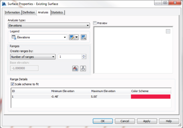
Figure 4.43 The Surface Properties dialog after manual editing
- Click Apply to apply the settings in the Surface Properties dialog and the surface.
- Drag the Surface Properties dialog to the side. Notice the red solid fill in the ditch areas indicating elevations equal to or less than the maximum elevation entered.
- Back on the Analysis tab in the Surface Properties dialog, change the Maximum Elevation value to 6 (1.5 for metric users) and click Apply.
- Review the drawing area for the expansion of the red fill indicating elevations equal to or less than 6 (or 1.5 for metric users).
- Repeat steps 19 and 20 for a maximum elevation of 7 (or 2 for metric users).
- Click OK to close the Surface Properties dialog.
- Save the drawing for use in the next exercise.
Understanding surfaces from a vertical direction is helpful, but many times the slopes are just as important. In the next section, you'll take a look at using the slope analysis tools in Civil 3D.
Slopes and Slope Arrows
Beyond the bands of color that show elevation differences in your models, you also have tools that display slope information about your surfaces. This analysis can be useful in checking for drainage concerns, meeting accessibility requirements, or adhering to zoning constraints. Slope is typically shown as areas of color similar to the elevation banding or as colored arrows that indicate the downhill direction and slope. In this exercise, you'll look at the existing surface and run the two slope analysis tools:
- Continue working in the
0412_SurfaceAnalysis.dwgfile (or the0412_SurfaceAnalysis_METRIC.dwgfile). - Select the surface on your screen to activate the contextual tab.
- From the Existing Surface contextual tab Modify panel, click the Surface Properties icon.
- On the Information tab, change the Surface Style field to Slope Banding (2D).
- Switch to the Analysis tab of the Surface Properties dialog.
- Choose Slopes from the Analysis Type drop-down list.
- Set the Number field in the Ranges area to 6 and click the Run Analysis arrow in the middle of the dialog to populate the Range Details area.

The Range Details area will populate. You could change the minimum and maximum values as you did in the previous exercise, but this time you'll keep the defaults.
- Click OK to close the dialog.
The colors are nice to look at, but they don't mean much, and slopes don't have any inherent information that can be portrayed by color association. To make more sense of this analysis, you'll add a legend table.
- Select the surface again, and on the Existing Surface contextual tab Labels & Tables panel, choose Add Legend.
- At the
Enter table type [Directions Elevations Slopes slopeArrows Contours Usercontours Watersheds]:prompt, enter S ↲ to select Slopes. - At the
Behavior [Dynamic Static]: <Dynamic>prompt, press ↲ again to accept the default value of a Dynamic legend. - At the
Select upper left corner:prompt, pick a point onscreen to draw the legend, which is shown in Figure 4.44.
Figure 4.44 The slopes legend table
By including a legend, you can make sense of the information presented in this view. Because you know what the slopes are, you can also see which way they go.
- Select the surface, and on the Existing Surface contextual tab Modify panel, choose the Surface Properties icon.
The Surface Properties dialog appears.
- On the Information tab, change the Surface Style field to Slope Arrows.
- Switch to the Analysis tab of the Surface Properties dialog.
- Choose Slope Arrows from the Analysis Type drop-down list.
- Verify that the Number field in the Ranges area is set to 6, and click the Run Analysis arrow in the middle of the dialog to populate the Range Details area.

- Click OK to close the dialog.
The benefit of arrows is in looking for “birdbath” areas that will collect water. These arrows can also verify that inlets are in the right location, as shown in Figure 4.45. Look for arrows pointing to the proposed drainage locations and you'll have a simple design-verification tool.

Figure 4.45 Slope arrows pointing to a proposed inlet location
When this exercise is complete, you can close the drawing. A finished copy of this drawing is available from the book's web page with the filename 0412_SurfaceAnalysis_FINISHED.dwg or 0412_Surface Analysis_METRIC_FINISHED.dwg.
With these simple analysis tools, you can show a client the areas of their site that meet their constraints. Visually compelling and simple to produce, this is the kind of information that a 3D model makes available. Beyond the basic information that can be represented in a single surface, Civil 3D also contains a number of tools for comparing surfaces. You'll compare this existing ground surface to a proposed grading plan in the next section.
Visibility Checker
The Zone Of Visual Influence tool allows you to explore what-if scenarios. In this example, a 40' (12 m) tower has been proposed for the site. A concerned neighbor wants to make sure that it won't obstruct their scenic view. You want to check it from the proposed surface:
- Open
0413_VisibilityCheck.dwgor0413_VisibilityCheck_METRIC.dwg. - In Prospector, expand the Surfaces branch, right-click the FG surface, and choose the Select option.
- On the TIN Surface contextual tab Analyze panel, choose Visibility Check Zone Of Visual Influence.
- At the
Specify location of object:prompt, use the Intersection Osnap to select the center of the proposed tower located on the southern portion of the site (denoted by a large white square with an X inside). - At the
Specify height of object:prompt, enter 40 ↲ to set the tower height to 40' (metric users, enter 12 ↲). - At the
Specify the radius of vision extent:prompt, pan to and select the endpoint at the upper-right corner of the cyan-colored house located at the northeastern corner of the site.Save the drawing and keep it open for the next portion of the exercise.
The drawing now has bands of color:
- Green near the tower location indicates that the object is completely visible.
- Yellow indicates that the object is partially visible.
- Red indicates that the object is not visible.
So in our example, the homeowner on the upper right will be happy to know that the proposed 40' tower will not appear in their view.
In the next portion of this exercise, you will use the Point To Point tool.
- Using the same drawing, zoom to the intersection of Syrah Way and Cabernet Court, where you will see a car driving on the right side of the road.
You want to check the sight distance.
- If it is not already selected, select the FG surface.
- On the TIN Surface contextual tab Analyze panel, choose Visibility Check Point To Point.
- At the
Specify height of eye:prompt, enter 3.5 ↲ (metric users enter 1 ↲).This sets the height of the eye of a driver sitting in a typical car.
- At the
Specify location of eye:prompt, click where the driver would normally be seated in the vehicle. - At the
Specify height of target:prompt, enter 6 ↲ (metric users enter 1.8 ↲).A rubber-banding sightline ray appears.
- Click along the path where oncoming cars would be seen.
A sightline arrow is drawn on the screen:
- If the arrow is green, it means that the view is unobstructed, and the command line will tell you the distance from the eye.
- If any portion of the arrow is red, it indicates that the view is obstructed, and the command line will tell you the distance at which the obstruction occurs.
When this exercise is complete, you can close the drawing. A finished copy of this drawing is available from the book's web page with the filename 0413_SurfaceVisibility_FINISHED.dwg or 0413_SurfaceVisibility_METRIC_FINISHED.dwg.
Unfortunately, these visual tools are not dynamic; if you change the surface, you will need to rerun the visual tools.
Comparing Surfaces
Civil 3D contains a number of surface analysis tools designed to calculate earthwork quantities, and you'll look at them in the following sections. First a simple comparison provides feedback about the volumetric difference, and then a more detailed approach enables you to perform an analysis on this difference.
For years, civil engineers have performed earthwork using a section methodology. Sections were taken at some interval, and a plot was made of both the original surface and the proposed surface. Comparing adjacent sections and multiplying by the distance between them yields an end-area method of volumes that is generally considered acceptable. The main problem with this methodology is that it ignores the surfaces in the areas between sections. These areas could include areas of major change, introducing some level of error. In spite of this limitation, this method worked well with hand calculations, trading some accuracy for ease and speed.
With the advent of full-surface modeling, more precise methods became available. By analyzing both the existing and proposed surfaces, a volume calculation can be performed. Keep in mind that the quality of the result is highly dependent on the quality of the input surfaces. At every TIN vertex in both surfaces, a distance is measured vertically to the other surface. These delta amounts can then be used to create a third dynamic surface called a volume surface, which represents the difference between the two original surfaces.
TIN Volume Surface
Using the volume utility for initial design checking is helpful, but quite often contractors and other outside users want to see more information about the grading and earthwork for their own uses. This requirement typically falls into two categories: a cut-fill analysis showing colors or contours or a grid of cut-fill tick marks.
Color cut-fill maps are helpful when reviewing your site for the locations of movement. Some sites have areas of better material or can have areas where the cost of cut is prohibitive (such as rock). In this exercise, you'll use two of the surface analysis methods to look at the areas for cut-fill on your site:
- Open the
0414_VolumeSurface.dwgor0414_VolumeSurface_METRIC.dwgfile. - From the Analyze tab Volumes And Materials panel, choose the Volumes Dashboard icon to display the Volumes Dashboard in Panorama.
- Click the Create New Volume Surface button to display the Create Surface dialog.


Notice that Type is already set to TIN Volume Surface. You also have the option to select Grid Volume Surface. - Change the name to Pond Volume and set the style to Elevation Banding (2D).
- Click the <Base Surface> field next to Base Surface to display the ellipsis button.
- Click the ellipsis to select the Existing Surface and then click OK.
- Click the <Comparison Surface> next to Comparison Surface to display the ellipsis button.
- Click the ellipsis to select the Pond surface and click OK.
The Create Surface dialog should now look similar to Figure 4.46.
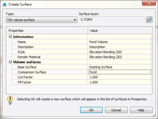
Figure 4.46 Creating a volume surface
- Click OK to accept the settings in the Create Surface dialog.
Civil 3D will calculate the volume (Figure 4.47). If the Event Viewer opens, click the green check mark in the upper-right corner of the dialog.

Figure 4.47 Composite volume calculated
Note that you can scroll right and left in Panorama to display additional information, including the ability to apply a cut or fill factor by typing directly into the cells for these values.
This new volume surface appears in Prospector's Surfaces collection, but notice that the icon is slightly different, showing two surfaces stacked on each other.
- Leave Panorama open, and in Toolspace Prospector, expand Surfaces, right-click Pond Volume, and select Surface Properties.

- On the Analysis tab, change Number Of Ranges to 2 and click the Run Analysis button.

- Change Maximum Elevation to 0 for ID 1 and Minimum Elevation to 0 for ID 2.
According to the color scheme, the cut will now be displayed in red, and the fill will be displayed as purple.
- Click OK to close the Surface Properties dialog.
- In Prospector, expand the Surfaces Pond Definition branches.
- Right-click Edits and select the Raise/Lower Surface option.
- Enter
-0.25at the command line to drop the pond 3” (metric users enter-0.075).Notice that a yellow exclamation point status flag has appeared next to the volume surface in Panorama as well as in Prospector. Panorama no longer lists the volumes and instead states “Out of date.”
- Right-click the Pond Volume surface in Panorama and select the Rebuild option.
- Right-click the Pond Volume surface again and select Surface Properties.
- On the Analysis tab, click the Run Analysis button to rerun the analysis.
Notice the minimum and maximum elevations update.
- Change Maximum Elevation for ID 1 and Minimum Elevation for ID 2 to 0 and click OK to update the color mapping.
- In Prospector under the Definition branch of the Pond surface, click Edits, right-click the Raise/Lower edit in the preview area, and select Delete.
A dialog will appear warning you that the selected definition item will be permanently removed from the surface.
- Click OK.
- Return to Panorama, right-click the Pond Volume surface, and select Rebuild All to return the original volume calculation.
- Close Panorama when complete.
- In Prospector, right-click Pond Volume in the Surfaces branch and select the Surface Properties option.
The Surface Properties dialog appears.
- In the Surface Properties dialog, switch to the Statistics tab and expand the Volume branch.
The value shown for Net Volume (Unadjusted) is the same as that shown in Panorama in the first part of this exercise.
- In the Surface Properties dialog, switch to the Analysis tab for the Elevations analysis type.
- Verify that Create Ranges By is set to Number Of Ranges and that the value is set to 3; then click the Run Analysis button to populate the Range Of Details area.
- Change Maximum Elevation for ID 2 and Minimum Elevation for ID 3 to 0.25 (or 0.08 for metric users).
- Change Maximum Elevation for ID 1 and Minimum Elevation for ID 2 to -0.25 (or -0.08 for metric users).
- Modify your color scheme by double-clicking the color to be modified.
The recommended colors are red, yellow, and green, where red indicates the worst-case cut, green represents the worst-case fill, and yellow represents a balance.
Figure 4.48 shows the completed elevation analysis settings.
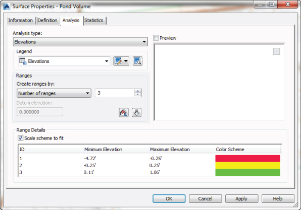
Figure 4.48 Elevation analysis settings for earthworks
- Click OK to close the Surface Properties dialog.
Save the drawing and keep it open for the next portion of the exercise.
The volume surface now indicates areas of cut, areas of fill, and areas that are nearly balanced, similar to Figure 4.49.

Figure 4.49 Completed elevation analysis
To show where large amounts of cut or fill could incur additional cost (such as compaction or excavation protection), you would simply modify the analysis range as required.
The Elevation Banding surface is great for onscreen analysis, but the color fills are too dense for most plotting purposes and can slow down the performance of the drawing. In the next steps, you use the Contour Analysis tool to prepare cut-fill contours in these same colors.
- In Prospector, right-click Pond Volume in the Surfaces branch and select the Surface Properties option to display the Surface Properties dialog again.
- On the Analysis tab, choose Contours from the Analysis Type drop-down list.
- Verify that the Number field in the Ranges area is set to 3 and click the Run Analysis arrow in the middle of the dialog to populate the Range Details area.
- Change the ranges to match those you entered in the previous portion of the exercise (as shown in Figure 4.48).
- In the Major and Minor Contour columns, click the small button to the far right of each to display the AutoCAD Select Color dialog, and set a color for each ID.

Typical contour colors are as follows:
- Shades of red for cut
- A yellow for the balance line
- Shades of green for fill
- Switch to the Information tab on the Surface Properties dialog and change the Surface Style to Contours 1' and 5' (Design) or Contours 0.5m and 2.5m (Design).
- Click the down arrow next to the Style field and select the Copy Current Selection option.

The Surface Style Editor appears.
- On the Information tab, change the Name field to Contours 0.25' and 1.25' (Earthworks) or Contours 0.15m and 0.75m (Earthworks).
- On the Contours tab, expand the Contour Ranges branch.
- Change the value of the Use Color Scheme property to True.
It's okay to ignore the range values here because you already set them in the surface properties.
- Expand the Contour Intervals branch and change Minor Interval to 0.25 (or 0.15 for metric users).
The Major Interval setting will automatically update to 5× the Minor Interval value.
- Click OK to close the Surface Style Editor and click OK again to close the Surface Properties dialog.
When this exercise is complete, you can close the drawing. A finished copy of this drawing is available from the book's web page with the filename 0414_VolumeSurface_FINISHED.dwg or 0414_VolumeSurface_METRIC_FINISHED.dwg.
The volume surface can now be analyzed on a lot-by-lot basis or labeled using the surface-labeling functions to show the depths of cut and fill, which you'll look at in the next sections.
Labeling the Surface
![]()
Once the three-dimensional surface model has been created, it is time to communicate the model's information in various formats. This includes labeling contours, creating legends for the analysis you've created, adding spot labels, or labeling the slope. These exercises work through these main labeling requirements and building styles for each.
Contour Labeling
The most common requirement is to place labels on surface-generated contours. In Land Desktop, this was one of the last steps because a change to a surface required erasing and replacing all the labels. Once labels have been placed, their styles can be modified.
Contour labels in Civil 3D are created by special lines that understand their relationship with the surface. Everywhere one of these lines crosses a contour line, a label is placed. This label's appearance is based on the style applied and can be a major, minor, or user-defined contour label. Each label can have styles selected independently, so using some AutoCAD selection techniques can be crucial to maintaining uniformity across a surface.
In this exercise, you'll add labels to your surface and explore the interaction of contour label lines and the labels themselves:
- Open the
0415_SurfaceLabeling.dwgor0415_SurfaceLabeling_METRIC.dwgfile. - Select the EG surface in the graphic to display the TIN Surface contextual tab.
- From the TIN Surface contextual tab Labels & Tables panel, choose Add Labels Contour – Single.
- Pick any spot on a major contour to add a label.
- Press ↲ when complete and press Esc to deselect the surface.
- From the Annotate tab Labels & Tables panel, choose Add Labels Surface Contour – Multiple.
- Pick a point to the west of the site and then a second point to the south of the site, crossing a number of contours in the process.
- Press ↲ to end the picking.
- From the Annotate tab Labels & Tables panel, add Surface Labels to display the Add Labels dialog.
- Verify that Feature is set to Surface and Label Type to Contour – Multiple At Interval.
- Click the Add button.
- Pick a point to the west of the site and then a second point to the north of the site.
- At the
Interval along contour <100.00>prompt, enter200(for metric60) at the command line for an interval value.Save the drawing and keep it open for the next portion of the exercise.
You've now labeled your site in three ways to get contour labels in a number of different locations. You will need additional labels in the northeast and southwest to complete the labeling because you did not cross these contour objects with your contour label line.
The contour label line is a handy tool. It has grips you can use to stretch it over other contours, which produces additional labels. You can also stretch it for the purpose of relocating labels. You can also copy the label line to other locations. Using the Properties dialog, you can turn it off, or you can turn it off by default on the Settings tab
Surface branch in Feature Settings. However, if a contour label is selected, the grips will reveal, and you can still use them to manipulate the position of the label.Next, you'll fill in the labeling to the northeast.
- Zoom to the northeast portion of the site, and notice that some of the contours are labeled only along the boundary or not at all, as shown in Figure 4.50.

Figure 4.50 Contour labels applied
- Zoom in to any contour label placed using the Contour – Multiple At Interval button and pick the text.
Three grips will appear. The original contour label lines are quite apparent, but in reality, every label has a label line beneath it.
- Grab the northernmost grip and drag across an adjacent contour northeast of the original label, as shown in Figure 4.51.

Figure 4.51 Grip-editing a contour label line
New labels will appear everywhere your dragged line now crosses a contour.
- Drop the grip somewhere to create labels as desired. Be sure to press Esc a few times when you have finished labeling the contours to end the command.
Save the drawing and keep it open for the next portion of the exercise.
By using the created label lines instead of adding new ones, you'll find it easier to manage the layout of your labels.
Additional Surface Label Types
With Civil 3D's surface modeling, spot labels are dynamic and react to changes in the underlying surface. By using surface labels instead of points or text callouts, you can generate a grading plan early on in the design process and begin the process of creating sheets. In the following sections, you'll label surface slopes in a couple of ways, create a single spot label for critical information, and conclude by creating a grid of labels similar to the labels in many estimation software packages.
Labeling Slopes
Beyond the specific grade at any single point, most grading plans use slope labels to indicate some level of trend across a site or drainage area. Civil 3D can generate the following two slope labels:
- One-Point Slope Labels One-point slope labels indicate the slope of an underlying surface triangle. These work well when the surface has large triangles, typically in pad or mass grading areas.
- Two-Point Slope Labels Two-point slope labels indicate the slope trend on the basis of two points selected and their locations on the surface. A two-point slope label works by dividing the surface elevation difference between the points by the planar distance between the pick points. This works well in existing ground surface models to indicate a general slope direction but can be deceiving in that it does not consider the terrain between the points.
In this next exercise, you'll apply both types of slope labels:
- Continue working in
0415_SurfaceLabeling.dwgor0415_Surface Labeling_METRIC.dwg. It is not necessary to have completed the previous exercise before proceeding. - Select the surface to display the TIN Surface contextual tab.
- From the TIN Surface contextual tab Labels & Tables panel, choose Add Labels Slope.
Alternatively, you can go to the Annotate tab
Labels & Tables panel and choose Add Labels Surface Slope. - At the
Create Slope Labels or [One-point Two-point]: <One-point>prompt, press ↲ to select the default one-point label style. - Zoom in on the circle drawn on the western portion of the site and use a Center Osnap to place a label at its center, similar to that shown in Figure 4.52.

Figure 4.52 A one-point slope label
- Press Esc or ↲ to exit the command.
- From the TIN Surface contextual tab Labels & Tables panel, choose Add Labels Slope.
- At the
Create Slope Labels or [One-point Two-point]: <One-point>prompt, enterT↲ to switch to a two-point label style. - Pan to the central portion of the site and use an Endpoint Osnap to pick the left end of the line.
- Use an Endpoint Osnap to select the right end of the line to complete the label.
- Press Esc or ↲ to exit the command and view the label, shown in Figure 4.53.

Figure 4.53 A two-point slope label
- Continue working in
This second label indicates the average slope of the property. By using a two-point label, you get a better understanding of the trend as opposed to a specific point. Please note when using the two-point label command, the arrow in the label points in the direction of the second point picked.
When this exercise is complete, you can close the drawing. A finished copy of this drawing is available from the book's web page with the filename 0415_SurfaceLabeling_FINISHED.dwg or 0415_SurfaceLabeling_METRIC_FINISHED.dwg.
Surface Grid Labels
Multiple labels placed in a grid pattern on the plan can be a huge help for grading contractors and estimators. In this exercise, you'll use the volume surface you generated earlier in this chapter to create a set of surface labels on a volume surface that reflect depth of cut and fill:
- Open the
0416_GridSurfaceLabels.dwgfile (or the0416_GridSurfaceLabels_METRIC.dwgfile). - From the Annotate tab Labels & Tables panel, choose Add Labels Surface Spot Elevations On Grid.
- At the
Select a surface <or press enter key to select from list>:prompt, select one of the surface triangles and click OK. - At the
Specify a grid basepoint:prompt, pick a point southwest of the Pond Volume surface to set a base point for the grid. - At the
Grid rotation:prompt, pick a point to the right that defines a line relatively parallel to the surface. - At the
Grid X spacing:prompt, enter25↲ (7↲ for metric users). - At the
Grid Y spacing:prompt, enter25↲ (7↲ for metric users). - At the
Specify the upper right location for the grid:prompt, pick a point northeast of the Pond Volume surface to set the area for the labels. - Verify that the preview window encompasses the Pond Volume surface, and press ↲ at the command line to continue.
Back at step 4, a triangle edge from Existing Surface was selected. Therefore, the resulting labels are displaying elevations of this surface instead of depth labels of the Pond Volume surface. Beginning with Civil 3D 2015, you can now change the object a label is referencing.
- Click a label, right-click, and choose Select Similar.
- Type PR ↲ to open the Properties palette.
- On the Properties palette under the second General section, double-click the value field next to Surface to change the surface being referenced by the labels to the Pond Volume surface.
- Press Esc to deselect the elevation labels.
Your drawing should look similar to Figure 4.54. Incidentally, any labels placed over Existing Surface that do not coincide with Pond Volume will appear as question marks. These can be deleted.

Figure 4.54 Volume surface with grid labels
When this exercise is complete, you can close the drawing. A finished copy of this drawing is available from the book's web page with the filename 0416_SurfaceGridLabels_FINISHED.dwg or 0416_SurfaceGridLabels_METRIC_FINISHED.dwg.
Point Cloud Surfaces
A point cloud is a huge bunch of 3D points, usually collected by laser scanner or Light Detection and Ranging (LiDAR). In a geographic information system, point clouds are often used as a source for a Digital Elevation Model. The technology has gotten less expensive and more accurate over the last few years, allowing LiDAR to quickly take over from traditional methods of collecting photogrammetry data.
Point clouds in many formats can be imported to Civil 3D. The most common format is the Log ASCII Standard (LAS) file. This binary format is a public format and at minimum contains x, y, and z data. LAS format can also include color, classification, and other information. For more information on the LAS standard, visit www.asprs.org.
Civil 3D can import a point cloud and use it in several ways. For instance, a laser scan of a bridge can be imported and placed for reference when you're designing a road through an existing abutment. In the example that follows, you will convert LiDAR data into a Civil 3D surface. It is important to note that point clouds often contain millions of points and may require a high-performance computer (and a little patience on your part) to process.
Importing a Point Cloud
A typical point cloud contains millions of points. These large files are kept external to Civil 3D in a point cloud database. After the LAS has been imported, the data is passed to three files: PRMD, IATI, and ISD. The ISD file contains the points themselves and is the only file needed by CAD if the point cloud would need to be re-created or used in base AutoCAD. By default, these files get created in the same directory as the DWG, but the location can be changed when importing the information.
If the point cloud you are working with contains coordinate system information (as all the examples in this book do), the software will automatically convert the point cloud to the units and coordinate system of the drawing. For the exercises in this chapter, it does not matter whether you choose the Metric or the Imperial template.
Civil 3D may take a long time to process these files, and you must ensure that you have sufficient disk space to store them, as you will find in the following exercise. It is also a good idea to close the software and then reopen it to help clear some memory before starting memory-intensive tasks such as working with point clouds.
The following exercise will show you how to import and work with a point cloud:
- Start a new file by using the default Civil 3D template of your choice. Save the file before proceeding as
0417_PointCloud.dwg. - Imperial users, set the coordinate system to UTM with NAD83 datum, Zone 17, US Foot; Central Meridian 81d W (UTM83-17F). Metric users, set the coordinate system to UTM with NAD83 datum, Zone 17, Meter; Central Meridian 81d W (UTM83-17).
- In Prospector, right-click the Point Clouds branch and select the Create Point Cloud option to display the Create Point Cloud Wizard, shown in Figure 4.55.
- Set the name of the point cloud to Serpent Mound.
- Set Point Cloud Style to Elevation Ranges, as shown in Figure 4.55, and click the Next button.

Figure 4.55 The Create Point Cloud – Information page
The Source Data page is displayed, as shown in Figure 4.56.

Figure 4.56 The Create Point Cloud – Source Data page
- Using the white plus sign, browse to the
0417_Serpent Mound.lasfile, select it, and click Open (both Imperial and metric users can use this file).Remember, you can download all data and drawing files for this book from
www.sybex.com/go/masteringcivil3d2016.This is a large (90 MB) file containing roughly 1.4 million points and may require a minute or two to process.
- Once the file appears in the Source Data page of the wizard, click the Next button to display the Summary page, shown in Figure 4.57.

Figure 4.57 The Create Point Cloud – Summary page
- Accept the defaults, as shown in Figure 4.57, and click Finish to process the point cloud.
- If the New Point Cloud Database – Processing In Background dialog appears, click Close to dismiss it.
The components of the point cloud are being processed, including the graphic that will display in the lower-right corner of the application.
- Once the point cloud and surface is created, the Panorama will open displaying several warnings about duplicate points being ignored. Click the green check to close the Panorama.
When the exercise is complete, a portion of a bounding box outlining a portion of the point cloud is displayed in the center of the screen. Save the drawing, but leave it open to complete the next exercise. A finished drawing will not be provided because of the large file size.
Working with Point Clouds
Once the point cloud is visible in your drawing, you'll want to follow a few rules of thumb to prevent performance problems. The key-in POINTCLOUDDENSITY value controls what percentage of the full point cloud displays on the screen at once. You can also access this value using a slider bar in the Point Cloud contextual tab. However, it is easier to hit the percentage you want on the first try if you use the key-in value. The lower this value, the fewer the points that are visible; hence, the easier it will be to navigate your drawing. The POINTCLOUDDENSITY value does not have any effect on the number of points used when generating a surface model (this is similar to the Level Of Detail value used to aid surface processing).
When you are changing view directions on a point cloud, we recommend you use preset views and named views to flip around the object. The orbit commands should not be used because they are a surefire way to max out your computer's RAM. If you used the default template, your surface will be located on the V-SITE-SCAN layer. We suggest you freeze the layer if you do not need to see the point cloud. Use Freeze instead of Off for layer management so the point cloud is not accounted for during pan, zoom, and regen operations (this is true for all AutoCAD objects, but it makes a huge difference when working with point clouds).
Creating a Point Cloud Surface
By specifying either an entire point cloud or a small region of a point cloud, you can create a new TIN surface in your drawing. Any changes to the point cloud object will render the surface definition out of date. In the following exercise, a new TIN surface is created from the point cloud previously imported:
- Continue using the
0417_PointCloud.dwgfile you created in the previous exercise. - Select the bounding box representing the point cloud to display the Point Cloud: Serpent Mound contextual tab, shown in Figure 4.58.

Figure 4.58 The Point Cloud contextual tab
- From the Point Cloud contextual tab Point Cloud Tools panel, choose Add Points To Surface to display the Add Points To Surface Wizard, shown in Figure 4.59.

Figure 4.59 The Add Points To Surface – Surface Options page
- Name the surface Serpent Mound South. Leave the style set to the default.
- Click Next and the Region Options page is displayed (Figure 4.60).

Figure 4.60 The Add Points To Surface – Region Options page
- Choose the Window radio button and click Define Region In Drawing.
- Define the region by creating a window around the southern half of the point cloud.
- Click Next to see the Summary page, shown in Figure 4.61, and click the Finish button.
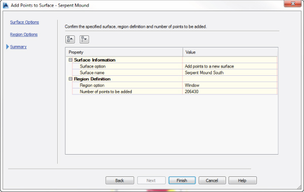
Figure 4.61 The Add Points To Surface – Summary page
Note that your number of points to be added will differ depending on the size of the window you created in the previous step.
When this exercise is complete, you can close the drawing. Because of the large file size, a finished state of this drawing is not available for download.
Surfaces created from point clouds behave in the same way as any other Civil 3D surface. You will see the point cloud source information in the Definition tab of Surface Properties. By default, the surface's existence depends on the point cloud. Because point clouds are so large, you may want to delete the point cloud from the drawing after the Civil 3D surface is created. If you choose to do this, be sure to set the Copy Deleted Dependent Objects option to Yes in the surface Definition tab. That way, once the point cloud has been removed, the surface will retain the point information.
The Bottom Line
- Create an existing ground surface using points. The most common way to create a surface model is by adding point data to the definition of a surface.
- Master It Open the
MasterIt0401.dwgor theMasterIt0401_METRIC.dwgfile. Create a new surface called Existing. Add the point group Topo to its definition. Leave the default styles.
- Master It Open the
- Modify and update a TIN surface. TIN surface creation is mathematically precise, but sometimes the assumptions behind the equations leave something to be desired. By using the editing tools built into Civil 3D, you can create a more realistic surface model.
- Master ItContinue working in the file from the previous exercise or open the
MasterIt0402.dwgor theMasterIt0402_METRIC.dwgfile. Use the irregular-shaped polyline and apply it to the surface as an outer boundary of the surface. Make the boundary a destructive breakline.
- Master ItContinue working in the file from the previous exercise or open the
- Prepare a slope analysis. Surface analysis tools allow users to view more than contours and triangles in Civil 3D. Engineers working with nontechnical team members can create strong, meaningful, analysis displays to convey important site information using the built-in analysis methods in Civil 3D.
- Master It Open the
MasterIt0403.dwgor theMasterIt0403_METRIC.dwgfile. Create a slope banding analysis showing slopes under and over 10 percent and insert a dynamic slope legend to help clarify the result of the analysis.
- Master It Open the
- Label surface contours and spot elevations. Showing a stack of contours is useless without context. Using the automated labeling tools in Civil 3D, you can create dynamic labels that update and reflect changes to your surface as your design evolves.
- Master It Open the
MasterIt0404.dwgor theMasterIt0404_METRIC.dwgfile. Label the major contours on the surface.
- Master It Open the
- Import a point cloud into a drawing and create a surface model. As laser scan data collection becomes more common and replaces other large-scale data-collection methods, the ability to use point clouds in Civil 3D is critical. Intensity helps postprocessing software determine the ground cover type. While Civil 3D can't do postprocessing, you can see the intensity as part of the point cloud style.
- Master It Import an LAS format point cloud file (
MasterIt0405_Denver.las) into the Civil 3D template of your choice. As you create the point cloud file, set the style to Elevation Ranges. Use a portion of the file to create a Civil 3D surface model. No coordinate system needs to be set for this example.
- Master It Import an LAS format point cloud file (