
Now it's time to use Gephi for creating and viewing a network where we begin to understand the spread of a contagious disease. It is critical to view more than a single network instance to best understand the contagion process. We'll view a single network at multiple points in time, given the temporal nature of infectious disease, to understand how nodes act within a specific time window (the contagious stage of the disease) in spreading the infection. As we noted earlier, even then, the spread of the disease is not inevitable, as it is dependent on the probability of transmission throughout a network.
Let's outline the necessary elements we'll need to build a useful contagion network:
- A network of nodes with some level of contact within a given period: For our example, let's set the number of nodes to
50, so we have some ability to view the spread of the disease without making our network overly complex. We'll use the Random Graph... generator in Gephi as a proxy for the sort of random contacts a network of individuals might encounter in a single day. - Several time-based (temporal) views of a single network: These views might contain the same member nodes in each case, or more realistically, an evolving network of nodes based on the time element. In this case, we'll take a look at a single network of contacts and assume a 72-hour period where each member node is susceptible to the disease. This will replicate the SIR model discussed earlier with each node falling into one of three states—susceptible, infected, or removed. We will also make the assumption that the duration of the infection is one day (24 hours), and any nodes that have previously been infected enter into the removed state after the infection period expires.
- A probability of disease transmission: This will be a number ranging between 0 and 1, with 0 representing no chance of transmission and 1 indicating a 100 percent transmission level. Let's set the threshold to 0.5 (50 percent) for our example.
This will give us a basic version for analyzing contagion within networks. For a more thorough discussion on contagion, there are many available resources, some of which are noted in the Appendix, Data Sources and Other Web Resources, of this book.
Let's start at the beginning of the 72-hour period, refer to this time as t0, and assume that a single node is infected, as shown by the dark coloring within the node. Susceptible nodes will remain lightly colored, while removed members will be depicted with no shading (note that none exist at the outset).
Here, we see the network at t0 as follows:
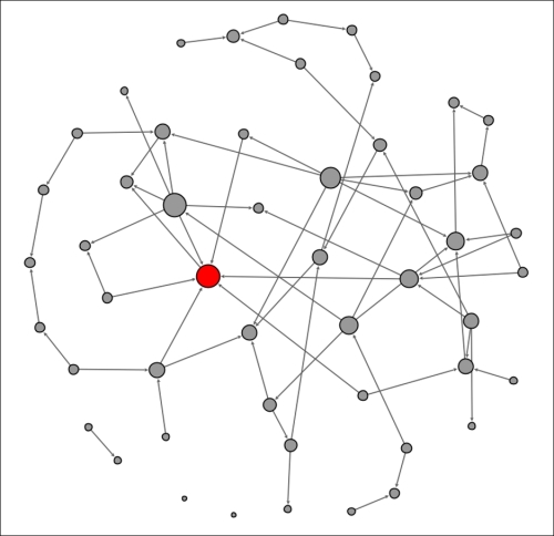
Contagion network at t0
Note the single node in an infected state. This individual is well-connected within the network, which will hasten the spread of the contagion. In this instance, there are seven direct contacts (assume that all these represent contacts made at t+1) of which approximately 50 percent will be infected. We'll assume that four of the seven are vulnerable to the infection, leaving us in this stage at the end of the first 24-hour period:
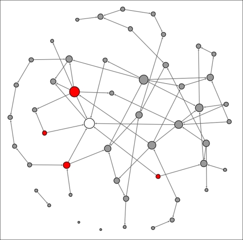
Contagion network at t+1
The original node that kicked off the contagion process is now removed from the eligible population, having already been infected, while the four newly infected nodes become the new transmitters of the disease. This process will repeat itself in the second 24-hour period (t+2) with the four infected nodes now immune and thus entering the removed state after having infected a new set of people:
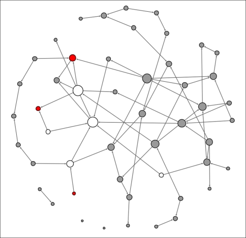
Contagion network at t+2
This is getting interesting, as we can see that some of the previously infected individuals have a few physical contacts, limiting the spread of the contagion. A few new nodes are now infected, but the disease is not spreading rapidly due to the limited contact levels. Finally, let's see what our network looks like at t+3:
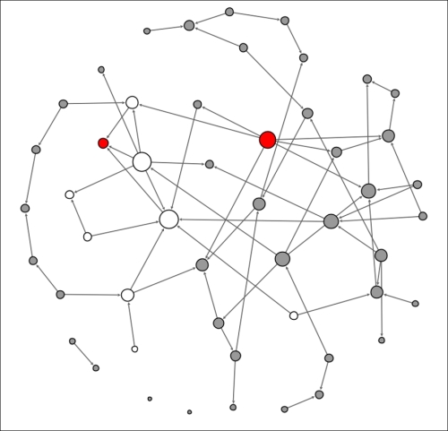
Contagion network at t+3
Note how the relative lack of contacts for some individuals managed to limit the spread of the contagion in our small network example. In the real world, this is certainly a possibility, but there is also a very high probability that the contagion will accelerate through densely connected networks, resulting in rapid spreading of the disease. This should help you understand how the structure of a network is critical to the transmission of many things, including infectious diseases.
I hope this provided you with some insight into how we can use Gephi to illustrate a simple contagion network. While this was a simple manual example, Gephi can be used with more comprehensive datasets with defined time periods and node statuses at each of these times. Some examples of this process are provided in Chapter 8, Dynamic Networks.