Earlier in this chapter, we discussed the concept of clustering in a network, and some of the ramifications for network structure and information flow. In this section, we'll use Gephi to provide you with some illustrations of networks with varying degrees of clustering, and add some further discussion on how Gephi can be leveraged to identify and measure clustering.

In the interest of clarity, I would like to take a moment to define clustering. When I refer to clustering in this section, it indicates the patterns that exist within a network, not the practice of creating clusters from the data. While the two instances are frequently related, this section is devoted to understanding why these patterns exist, and how they might affect the flow of information within a network. Later in this book we'll examine how to create clusters or partitions within the network through the use of defining characteristics in the data. These topics will be addressed in Chapter 7, Segmenting and Partitioning a Graph.

The best way to detect clustering within a network is to provide some visual examples of networks with varied levels of grouping, ranging from virtually none at all (a random network), all the way to a network with a high proportion of completed triangles, and confirming the presence of significant levels of clustering. Our key statistics to detect clustering can be found in the Statistics tab. We'll now use Gephi to present three examples that show detailed networks on low clustering, moderate clustering, and heavy clustering. This should help you quickly convey what we are looking for when we speak of clustering within a network.

For these examples, we'll use one of the Erdos-Renyi generators, which is found by navigating to the File | Generate | Erdos-Renyi G(n,m) model option. In each case, we'll set our network to 50 nodes while changing the number of edges from 100 to 200, and finally to 300. In doing so, we should anticipate higher levels of clustering as the number of edges grow. We'll begin with the graph of 50 nodes with just 100 edges—a rather sparse network:

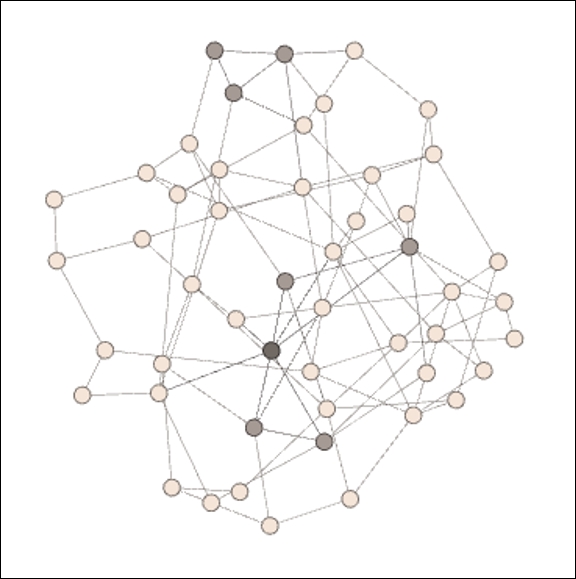
Erdos-Renyi network with low clustering

Note the presence of several colored nodes, indicating either one or two completed triangles. The vast majority of nodes have no complete triangles—the friends of a given node are typically not friends with one another. The average clustering coefficient for this network turns out to be just 0.022, which means that just over 2 percent of possible triangles are actually realized. When we increase the number of edges to 200, the network changes dramatically, as shown in the following diagram:

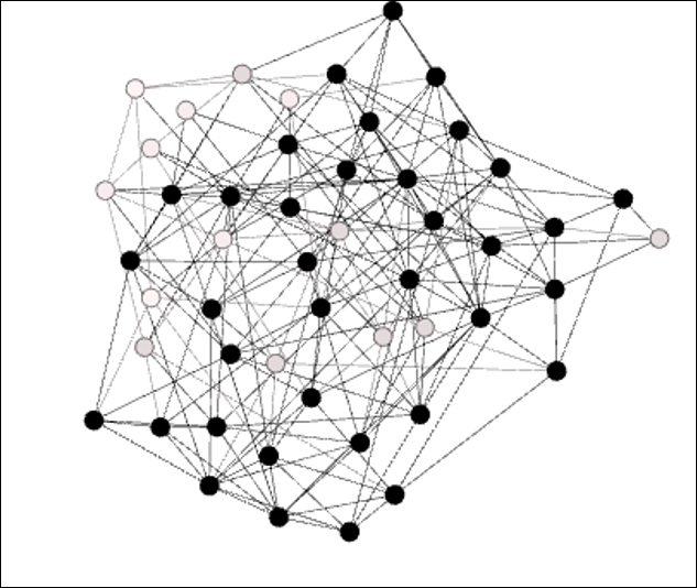
Erdos-Renyi network with significant clustering

We now see a much denser network, since the number of edges has doubled. This doubling has had an even more pronounced impact on clustering, as the average clustering coefficient has now grown to 0.164. One of every six possible triangles is now complete, compared to the one in 45 as seen in our first graph. The dark nodes indicate at least three completed triangles per member; note that there are just a couple of areas of the graph where the member nodes don't reach this threshold.

Finally, we'll take a look at the same model with 300 edges:

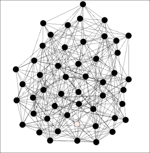
Erdos-Renyi network with high clustering

Our network is now growing quite dense with many members connected to each other. Note just a single node (at the center bottom) that falls short of the three completed triangle criteria from the prior graph. Being consistent with these patterns, we now have an average clustering coefficient of 0.253—one of every four possible triangles is complete.

We have used the clustering coefficients to tell us when clustering is present, but this has not shown us which nodes form communities based on the clustering patterns. For this, we can turn to a couple of options. Several Gephi plugins exist that can be used to detect clusters based on connection patterns and community structures. The Chinese Whispers plugin is a very capable option if we choose this path. For this example, we'll simply use the Modularity option found in the Network Overview section of the Statistics tab. After running this function, we can then apply the results as colors to our graph and get a very nice look at where the clusters exist. Let's take a look at our final Erdos-Renyi network:

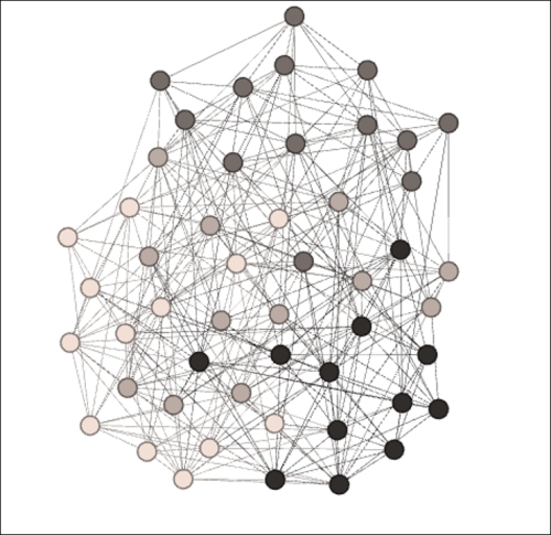
Clustering using the modularity function

Now we can see four distinct clusters ranging from light to dark. We see some limited overlap, but we can now easily view clustering patterns in the network. Cluster 4 (the darkest nodes) occupies the lower-right position, while Cluster 3 (the dark gray nodes) is dominant at the top of the graph. These relative positions might change depending on the algorithm used, but should remain visually distinct.

This last point is particularly important to understand our data; each algorithm will depict the data according to its particular settings. Even within each layout selection, we have multiple options for setting spacing through attraction and repulsion settings. This topic is covered in more detail in Chapter 3, Selecting the Layout. It is essential that you experiment with different settings so that your data conveys the story it was supposed to tell, and network clustering is a component of this process. If there are natural clusters within the network, graph viewers must be able to detect them. Otherwise, the graph conveys an incomplete if not an inaccurate story, which is something to avoid if at all possible. Better to not tell the story at all rather than be misleading.