
Complex filters, for our purposes, are defined as filters with two or more conditions placed on some combination of nodes, edges, partitions, or clusters, once again for the purpose of focusing on a specific set of elements within a larger network. Using multiple filters in Gephi is not always easy or intuitive, so we will spend some extra time in this section to walk through several examples in order to expose both the complex filtering approach and the potential for further use of complex filters in your own graphs.
Let's start with some relatively simple examples, complex only in having more than a single filter. In this case, we will create one filter and then use a second condition as a subfilter to the first. Here are the steps:
- Go to the Filters | Attributes | Equal filter and select the
classnameattribute. - Drag the filter to the Queries space in the lower half of the Filters tab.
- Type the value
3Bin the Pattern textbox and click on the OK button. You might also need to rerun the Select and Filter processes. - Now repeat step 1 using the
genderattribute and drag it to the subfilter area of the initial filter. - Enter the value
Fin the textbox and click on OK. Our settings should look like this: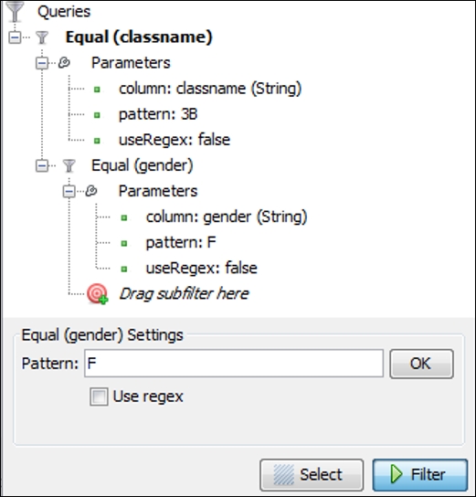
Using an equal filter with a subfilter
We should now see the following result in your graph window:
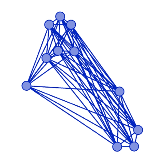
Nodes filtered by classname equals 3B and gender equals F
We now have a graph that has been quickly reduced to just 11 nodes of the original 236 by merging two simple filters. From here, we can easily change the classname value or the gender value that allow us to filter the network in a rapid fashion. This filter could also be saved for later use by right-clicking on and selecting Save, which will park the filter in the Saved queries folder. Let's move to another example; this time we will cover an example that combines three separate filters into a single query by using the subfilter capability.
This time we'll really narrow our graph down by merging three filters as follows:
- Go to the Filters | Attributes | Partition filter and select the
genderattribute. - Drag the filter to the Queries space in the lower half of the Filters tab.
- Select the F value by clicking on the adjacent rectangle and click on the Select and Filter buttons. You'll now see only female members of the network.
- Go to the Topology | Degree Range filter and drag it to the subfilter section of the gender filter we just created. Now adjust the value to a minimum of
60by using the left slider or by entering text. - Navigate to the Operator | NOT (Nodes) filter and drag that to the subfilter area of the degree range filter we just created.
- Go back to the Partition filter and select
classname. - Drag
classnameto the subfilter area of the NOT (Nodes) filter. - Run Select and Filter using the usual buttons.
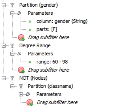
Here's what our filter should look like:
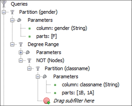
Complex filter that combines gender and degree range excluding the classnames 1A and 1B
We now have a filter that identifies all highly connected female members of the network who are not in classnames 1A or 1B. Here's our result:
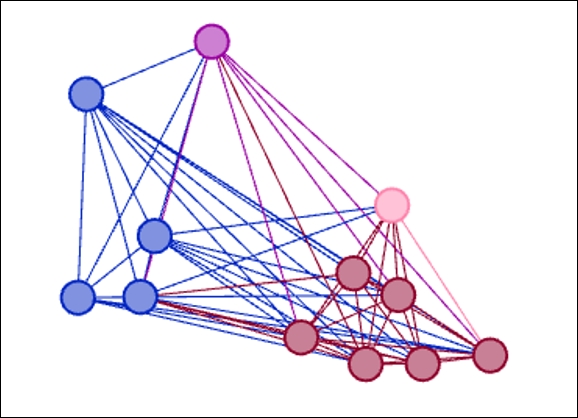
Results of filtering on female, degree range of 60-98, and not in 1A or 1B
You can see how quickly we whittled the network to just 12 nodes by combining these three conditions. From here it's also easy to tweak the settings—perhaps we would like to view only the 10 most connected female students. Simply increasing the degree range threshold will enable us to see these results refreshed with the new conditions. In fact, if we increase this value from 60 to 62, we are left with just nine students who meet all three criteria.
What would happen if we hadn't nested these criteria in a single query, but had chosen to isolate each filter? You can probably guess what the results will look like. Here are the three filter conditions we just presented, but now they act as standalone queries:
Individual filters not nested in a single query
To create this query, simply follow the same steps we previously used, with one exception. Rather than nesting each filter inside another as a subfilter, this time add each one as its own query, as shown in the preceding screenshot. Run them one at a time by clicking on the Select and Filter buttons.
First, we'll run the Partition filter with the value set to F, which results in the following graph:
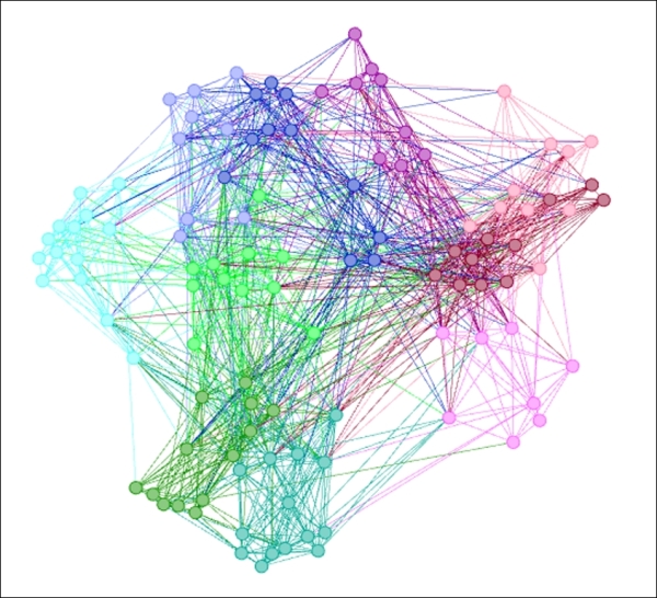
Filtering on partition equal to F
As you might have anticipated, the network has been reduced to roughly half by hiding all nodes with gender equal to male.
Next, we'll filter on Degree Range, to identify all network members ranging between 60 and 98 degrees. Make sure the lower value is set to 60, and then filter the results to see the following output:
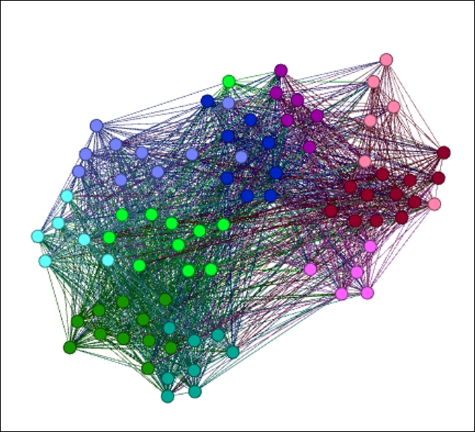
Filtering on degree range between 60 and 98
Now you are seeing only those nodes with a degree level of 60 or greater, including both male and female members. The prior filter is effectively overwritten by the new condition, rather than combining them as we previously saw. To verify that this is the case, go to Data Laboratory and view the results to confirm the presence of both male and female students.
Let's apply our third filter—the NOT (Nodes) operator that excludes classnames 1A and 1B. You should see the following results:
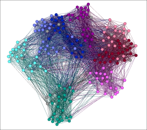
NOT (Nodes) with partition on classname equal to 1A and 1B
Not only do we have both genders visible in our dataset, but also students from the entire degree range from 18 through 98. The only missing members are those from classnames 1A and 1B, which can be confirmed by viewing the Data Laboratory results.
So while these individual filters can obviously not be used in the same manner as the nested versions, they do have a considerable value. If you wish to filter your network across many conditions then simply set those up in the Queries window, and then you have the ability to toggle through an array of filters to learn more about your network. Think of it in the same way as a statistician might work with single variable crosstabs to learn more about a dataset before moving on to a higher level of complexity.
Now let's tackle our remaining examples, starting with an instance where we will focus on the ego network of an individual student. To complete this example, we'll work with the INTERSECTION filter, found in the Operator folder within the Filters tab, as follows:
- Apply the Ego Network filter found in the Topology folder of the Filters tab. Follow the usual process of dragging the filter to the Queries tab, and then setting Node ID to
1551. Run the filter to get the initial results. This might appear a bit messy at this point, but we're going to take care of that in a moment. - Next, locate the MASK (Edges) filter found in the Operator folder of the Filters tab. Things get a bit trickier here, but we'll recap our steps at the end of this section. Drag the filter to the Queries tab as a standalone filter. Then add the
Idfilter from the Equal folder. Make sure you select the node version, rather than the edge filter. Add this to the subfilter area of the MASK (Edges) filter and set the value to1551, just as we did in our initial filter (we need these values to agree with one another). By the way, your graph will still look a bit untidy at this stage. - Next, repeat the process we just did with the
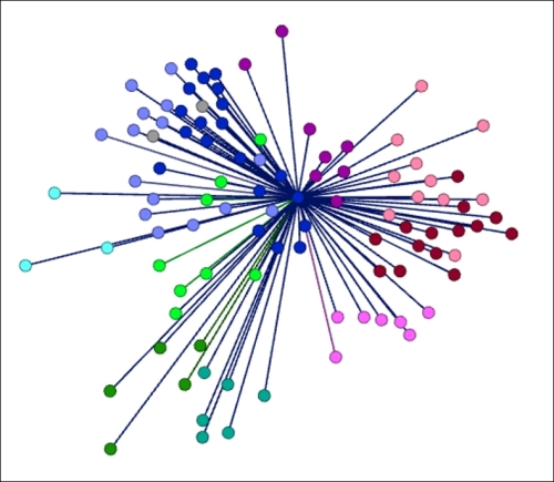
Id (Node)filter by dragging it to the subfilter section of the firstIdfilter. Set the value to1551yet again. Now your graph should look quite different—a network with many nodes (98 to be specific) but with no connecting edges. To make the edges appear, we need to create an intersection between our filter conditions. - To complete the process, drag the INTERSECTION filter from the Operator folder down to the Queries tab. Make sure it is standalone at this point. Then drag the original filters one at a time into the subfilter area of the INTERSECTION operator. Set the MASK (Edges) setting to any by selecting the corresponding radio button, and run the Select and Filter processes. If you have taken a look at an intermediate stage, you might have seen something along these lines, with extra nodes that are not part of the ego network:
Ego Network with masked edges, intermediate stage
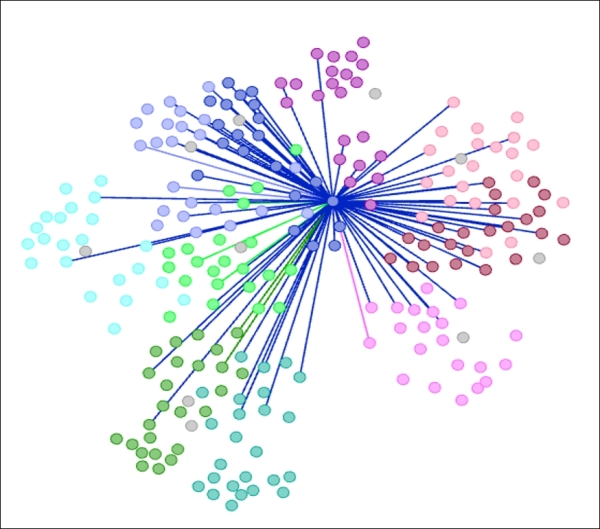
Your finished graph will resemble the following graph, with the remaining nodes filtered out of the process, and all first degree connections displayed like this:
Completed ego network with masked edges
Here's a screenshot for how your complete query will appear:
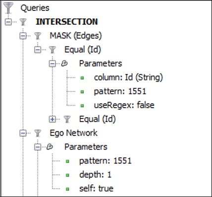
Intersection of masked edges and ego network
Remember to set the second (redundant) Equal (Id) value to make sure that the filter operates as expected. This might seem slightly quirky at first, but once learned, it becomes simple to apply to many other examples.
Now that we have run through a fairly complex example using the intersection logic, we'll end the chapter with an instance using the UNION operator. If you think of intersections as being parallel to the use of AND constructs in database queries, then unions are much closer to the OR condition. One notable difference is the requirement that union queries to get based on a single data attribute, where intersections derive their power from merging conditions across multiple attributes.
Given that this example is easier to follow than the last, we'll first introduce the filter conditions of the filter that we are creating, and then view the results. Here's how we want our filter to appear, which can be achieved by performing the following steps:
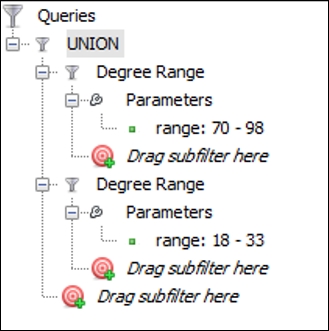
Union query with low and high degree ranges
To create the filter, follow these steps:
- Go to the Filters | Topology | Degree Range filter and drag it to the Queries tab.
- Repeat the same process by dragging the second filter to the Queries tab as a standalone instance.
- Set the first Degree Range filter to a minimum value of
70. - Set the second filter to a maximum value of
33. - Go to the Filters | Operator | UNION filter and drag it to the Queries tab as a standalone item.
- Drag each of the two filters to the subfilter area of the UNION operator, similar to what we did with the intersection example.
- Run the filter using the Select and Filter buttons.
Your result should look like this:
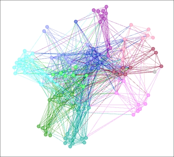
Results of union query on degree ranges
We now have a graph that shows the least connected members of the network, as seen near the perimeter of the graph, and the most highly connected nodes concentrated in the center. The results can be verified in the data laboratory, where we see no nodes with degree values greater than 33 or less than 70. We could follow a similar process using other data attributes such as classname.
I'm sure that you have also thought of some additional applications for complex filters using your own datasets, and it is my hope that these examples will provide both a springboard and reference for some of these processes.