
In this final section of the chapter, we're going to apply many of the statistics we've just reviewed to our school classroom data and begin to gain a greater understanding of the network beyond our earlier visual assessments. Even better, we will use the power of filtering in tandem with the graph statistics to begin using Gephi in an even more sophisticated fashion. We'll start this section with some fairly straightforward examples, and then move on to more complex analysis using the available filtering options.
We're going to work once again with the primary school dataset as we will illustrate the practical application of many of these statistics. We'll proceed in the following order:
- The first section will apply some of the network-oriented measures that will inform us about the general structure of the graph
- Our second section will view several of the centrality statistics and compare how individual nodes are classified
- We will close out by taking a look at a few of the clustering statistics in order to gain a better understanding of how individual nodes form groups based on their behaviors and location within the graph
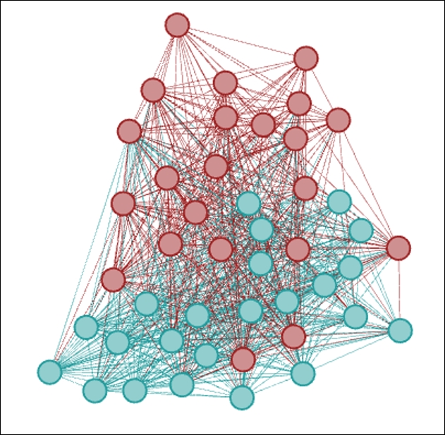
Let's begin by checking out a few of the network-based statistical measures, and what they tell us about our primary school data. We'll work through each of these statistics by providing the calculated values from the school network graph, and follow with discussions on the overall meaning of each measure. Before we begin, it might be helpful to see the network as follows:
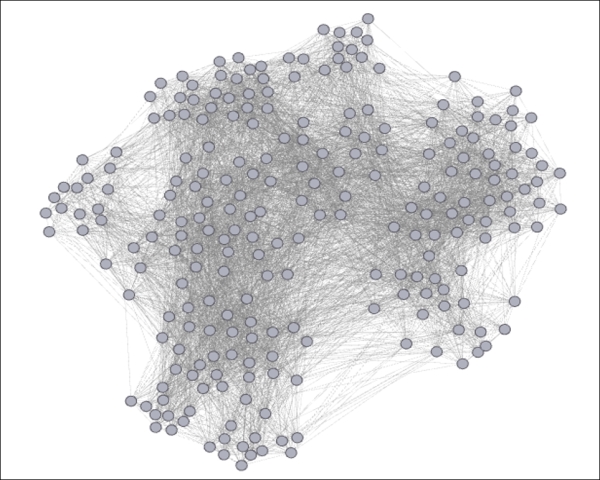
Primary school network
The several measures discussed in this section will provide a lens into the general structure of the network—its size, density, and efficiency will be examined as ways of understanding the composition of the graph. These statistics will help lay the groundwork for the more detailed centrality and clustering measures to follow. Remember that each of these statistics (and many others) can be found in the Statistics tab within Gephi. For most, all that is necessary is to click on the Run button. For a few others, you will need to specify whether your network is directed or undirected.
Let's see what results we get for some of the critical network statistics. You should be able to easily validate these numbers in your own Gephi instance.
The maximum steps required to cross the network is three, which would seem to indicate a network without a lot of clustering. This seems to be a fairly low value relative to the total number of nodes (236).
About 20 percent of the nodes have an eccentricity value of 2, with the remaining 80 percent requiring three steps to reach the furthest member of the graph. This provides further confirmation that this network is relatively evenly distributed and easily traversed by all nodes. We do not have any outliers at the fringes of the network who require four or five steps to cross the graph (this would require a higher network diameter, of course).
About 21 percent of nodes are connected with one another, based on the output value of 0.213. This is neither an exceptionally high number, nor could it be considered very low. If we reflect on the parameters of this network (grade levels, individual classes), the number appears to make sense in its context. The next step would be to compare this with the same measure from a similar network to judge whether this value is within an expected range (as it seems), or if this network is typically well connected or poorly connected.
It takes nodes close to two steps (1.86) on average to reach any other node in the network. This feels like a reasonable number given the prior measures we have discussed. If our graph density figure was considerably higher, we would then anticipate a lower average path length, as a higher proportion of members would have first degree connections.
As expected in a well-connected network, there are often multiple paths available to reach specific nodes, resulting in only a few edges with very high values; for instance, 97 percent of all edges have values below 0.5, with the range running between 0.34 and 1.0 The literal translation is that there are just 3 percent of cases where more than 50 percent of all nodes must travel along a single path to reach another node most efficiently (that is, shortest path). This informs us that we have a very robust network for information flow, and that even if a number of links were broken, the network would still be well-connected and efficient.
So what have we learned about the structure of this particular network?
- Overall, it seems safe to assume that this is generally a tightly knit network with minimal variation, as determined by eccentricity levels
- The network appears to be well-connected judging from the graph density measure, but it does not seem to be especially dense
Next, we'll look at a handful of centrality statistics from the same network, and determine what sort of story they are telling us about the behavior patterns of individual nodes inside the graph.
We previously talked about the use of centrality statistics for understanding the role played by each member of the network. In this section, we will also see how these measures help to define aggregate patterns within the graph and begin to understand how these individuals interact with one another. Our analysis will be based on four key centrality approaches: degree, closeness, eigenvector, and betweenness.
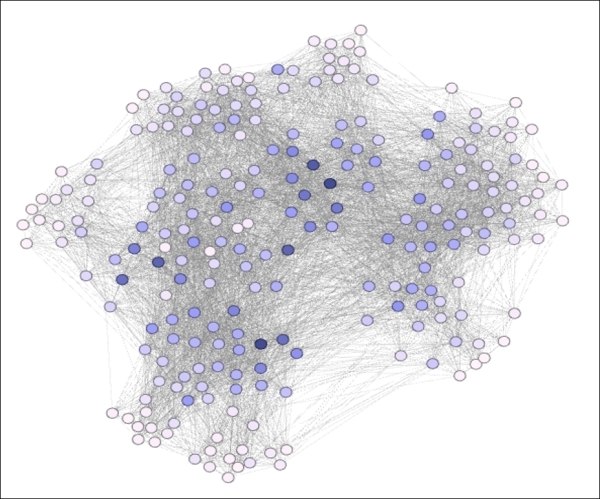
There is a considerable variation in the degree ranges within this network (from 18 through 98), as is the case in the majority of network graphs. This is not an extreme variation in the sense of measuring nodes on the Web, but given the total potential number of degrees (n-1 = 235), it does represent a significant variance. To help illustrate these differences, let's have a look at a graph where we have colored the nodes based on degree level—darker colors being indicative of higher degree counts:
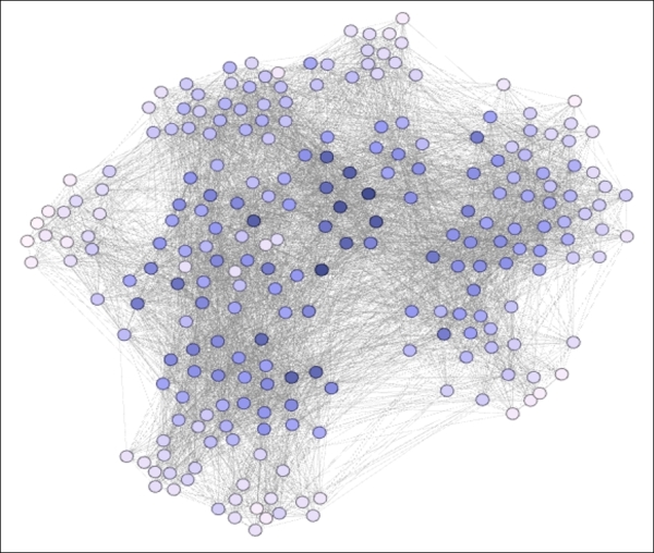
Degree centrality expressed using node coloring
We can now see how the high degree nodes tend toward the center of the graph, while those with low degree values are forced to the perimeter; a typical pattern for many layout algorithms. It is also evident that many of the high degree members are in close proximity to one another, an observation which will prove consistent with the lack of significant clustering in this network. This fact will also influence some of the other centrality measures.
This is a much tighter distribution (1.583 through 2.209) than we saw for degrees, largely attributable to the generally close-knit structure of this network. As you can recall, the eccentricity level for all nodes was either 2 or (mostly) 3, an indication that there are no far-flung outliers residing at a great distance from the center of the graph. In cases where there was a greater distribution of eccentricity, we would anticipate a more dispersed distribution of values for this statistic. Visually, this is what we see, again coloring the values based on the statistic, with higher closeness scores (that is, greater distance) indicated by darker nodes:
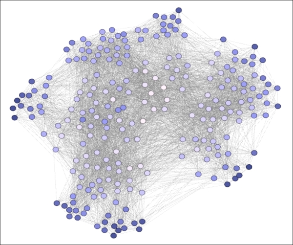
Closeness centrality expressed using node coloring
Remember that this is a sort of inverse measure—higher values indicate more distant levels of proximity to other members of the network. So the same nodes that had fewer direct connections are also associated with higher closeness measurements, which should come as no surprise. Those in the center of the graph can more easily travel to all other nodes in the network (on average), while members on the perimeter cannot do so quite so easily.
In contrast to the narrowly distributed values within the closeness centrality statistic, we see a far greater range for the eigenvector measurement (0.108 through 1). Now we are attempting to understand the relative importance of connections to gauge whether influential members are likely to be connected with other members of similar standing. Likewise, this measure will tell us whether nodes with lower influence are more likely to be connected with their peers. In this case, both of these patterns appear to be true, giving us a wide range of values. Our example looks like this:
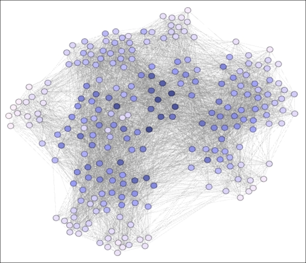
Eigenvector centrality expressed using node coloring
Here, we have a diagram that resembles, but differs slightly from the degree centrality image shown a moment ago. As expected, the higher levels of centrality are concentrated in the center of the graph, with a general progression toward lower levels as we approach the perimeter. Influential nodes are surrounded by other influential nodes, with the inverse also true, that is, low degree members are largely enmeshed with similarly behaving nodes.
There is a rather large spread in betweenness centrality from top to bottom (2.7 to 396.7), with a few nodes having values near zero located around the perimeter of the network. At the other extreme is a total of 8 nodes with betweenness measures of 300 or greater. These members are important players that help to connect diverse portions of the network, although we don't have any that fill the classic role of a bridge between clusters. A view of this statistic seems to confirm what we have already learned about the network:
Betweenness centrality expressed using node coloring
As expected, nodes at the perimeter have very low betweenness scores—there is nowhere to go that requires traveling through these members. However, we can detect a handful of critical members that facilitate network traversal, and notice how they are spread out to a much greater degree than we saw for some of the other measures. This is actually quite logical, as it would make little functional sense to have two nodes with very high betweenness properties sitting adjacent to one another; this would be highly redundant. Instead, we can see a more scattered pattern with one or two high scoring nodes strategically located within the graph, which help to create a more efficient network.
Based on these statistics, we can safely conclude the following:
- There is a high level of differentiation across individual nodes, as shown by the variance in degree level
- The most highly connected nodes tend to associate with one another, while lower degree members primarily link to similar sorts of nodes
- There is considerable differentiation in betweenness centrality, even though the network does not require bridge nodes
Our third and final section will examine a few of the clustering measures available in the Statistics tab, and what they can tell us about the behavior patterns within this network.
Our aim in interpreting the clustering statistics is to comprehend larger behaviors taking place within the network, to see if there are identifiable patterns that tell a significant story. Conversely, the lack of any evident clustering behaviors can also tell a story about the network. We'll analyze five key statistics in the context of our school network to unearth any patterns, beginning with the clustering coefficient.
As we discussed earlier, this is a measure that determines the percentage of available triplets that are fully closed. The statistical measures are 0.502 for the network, and 0.338 to 0.877 for individual nodes. In the case of our school network, the total network number is almost exactly half closed, with the remaining 50 percent still open—two of three edges are connected, but the third edge is missing.
Is this a high or low number? Again, this is somewhat subjective as well as dependent on the individual network, but it does seem to be a rather high figure. If we reflect back to what this network is measuring, this should not come as a complete surprise; we are not looking at long-term relationships or collaborations, but simply interactions between individuals within and across classrooms. The number will almost certainly grow if we restrict it to a single grade level or classroom, as it will reflect the proximity of members throughout the course of a day.
When we examine patterns at the individual member level, we see a wide range from less than 35 percent up to nearly 90 percent of all triplets being closed. Remember that this statistic is inversely correlated to the number of degrees and it begins to make sense. Nodes with relatively few connections are considerably more likely to have a high percentage of closed triplets, while the lowest coefficients come from some of the most aggressively connected members of the network.
There is a very wide range of triangles from the minimum (96) to maximum (1,616) number of triangles at the node level. At first, this variance seems extreme, but if we step back and look at a couple of other statistics, these numbers make complete sense. First, consider that our degree ranges ran from 18 to 98, and second, remember that many of the most popular nodes are connected with one another (the same is true for the least popular ones). This creates a geometric effect that favors the most highly connected nodes, at least in terms of the number of available triplets. However, as we learned from the clustering coefficient figures, a majority of these triangles will remain incomplete.
The modularity statistic splits this graph into five distinct clusters, numbered from 0 through 4. Doing some simple math tells us that each cluster will average close to 50 nodes. This might be satisfactory for our purpose, or if we need further splits, we can employ one of the dedicated clustering algorithms. A quick way to determine if this number is adequate is to color the graph using the modularity class, as we have previously done with the centrality measures.
This network has many Link Communities ranging in size from a single edge to well over 100 edges. What this tells us is not clear from a purely statistical viewpoint, but it can help us decipher interactions between multiple nodes, as defined by their connecting edges. In fact, the two most prominent communities in this graph account for greater than 20 percent of all connections, providing a new insight about the common behaviors that might be less clear if we rely solely on node-based statistics.
Our final clustering-oriented statistic to measure is embeddedness, which will aid us in understanding the depth at which nodes are affiliated with specific groupings. This measure can help explain how specific nodes or groups of nodes cooperate with one another beyond simply being superficially connected. In our school network, we have an average embeddedness level of 24.6 with individual edge values ranging from 0 to 64. If we examine the data further, it tells us that those edges with very low counts (infrequent interactions) are found at the lowest embeddedness levels; conversely, the highest scores typically correspond to frequent interactions between two nodes.
In the first case, this would represent the sort of superficial connection just referenced; perhaps this contact was random or incidental to a certain time and space. As the frequency of contacts between two parties grows (and with it, the embeddedness score) we can be fairly certain that this is not a random pattern, but something more purposeful and structured.
Now that you have learned how to work with a variety of useful statistics, it's time to take them to the next level by combining them with the powerful filtering capabilities in Gephi. We'll look at a number of graphs in this section so that you get a feel of both, the visual output of the various statistics as well as the multiplicative power delivered by the filtering capabilities of Gephi.
We spent a lot of time with filtering in the previous chapter prior to diving into graph statistics. Now we have an opportunity to combine these two powerful features in Gephi, as we can employ most of the statistical measures we have just reviewed as filters to help refine our graph output. This capability gives us considerable power to learn more about our network and drive attention to the most important aspects of the graph. We can also probe to understand the statistical variation within the network which might provide some surprises that would otherwise go unnoticed.
We'll use multiple graphs in this section to help illustrate the impact of combining statistics with filtering. So let's begin by working with some rather simple examples before stepping up the complexity level and showing some of the impressive capabilities of Gephi.
Let's begin with a simple case where we wish to focus our attention on only those nodes that meet a specified betweenness criteria; so we can better understand which nodes are most critical to connect sections of the network. If you recall, our betweenness levels ran from near zero all the way to nearly 400. We're going to follow a few steps to set a filter for only those nodes with betweenness levels above 250. While this number is slightly arbitrary, it is designed to identify the top 5 percent to 10 percent of the influential nodes. Refer to the paper Identifying High Betweenness Centrality Nodes in Large Social Networks, Nicolas Kourtellis et al, 2014, for more insight into identifying the impact of betweenness centrality.
This should give us a good sense for which members are most adept at connecting other nodes. Perform the following steps:
- Open the Filters tab in the Gephi workspace.
- Navigate to the Attributes | Range | Betweenness Centrality attribute.
- Drag the filter down to the Queries area.
- Set the lower range to
250using the slider control or type the value manually. - Click on Select and then Filter to get the results.
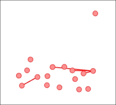
The original network of 236 nodes has now been dramatically reduced, as shown in the following graph:
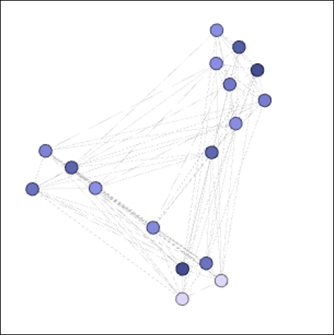
Nodes with betweenness centrality levels greater than 250
We now see the 17 most influential modes in terms of their ability to connect to others in the network. We can of course manipulate the filter to further reduce this group by raising the threshold, or to expand it by reducing the lower bound of the filter.
If you have been working along with these examples, you will have noticed many other statistics that are now available for filtering purposes. In addition to the various centrality measures, we now have the ability to look at hubs, triangles, neighborhoods, eccentricity, embeddedness, and communities, among others. We can also begin to apply some of the more advanced filtering techniques we worked with in the last chapter, giving us incredible power over the network. Let's take a look at a few of these possibilities.
We'll begin by merging the betweenness measure with a specific classname in order to understand which members are most likely to be the bridges within a given class. We're going to assume that you have already applied the previous filter. If not, you can start by following the last process of setting the Range filter using betweenness centrality:
- Set the lower bound of the range to
150. - Run the Select and Filter processes to verify the new setting.
- Navigate to the Attributes | Partition | classname variable.
- Drag this filter to the Queries window, as a separate filter and not a subfilter.
- Click on the 2B option in the Partition Settings window.
- Go to the Operator | INTERSECTION filter.
- Drag this to the Queries window, again as a separate filter.
- Move each of the prior filters under the INTERSECTION query as separate subfilters. Repeat steps 3 and 4 by dragging the classname filter to the subfilter area of the original classname filter.
- Apply the filter by running the Select and Filter processes.
We now have a new result that has merged our two filters by requiring a betweenness centrality of at least 150 combined with membership in classname 2B. I took the liberty of adding node labels, so we can see who these individuals are:
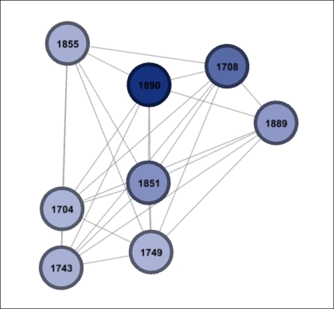
Intersection of betweenness and classname filters
If you wish to see additional details, simply navigate to Data Laboratory, which will now show only the results for these 8 nodes. Of course, if you wish to reduce this set, or apply the logic to a different classname, then simply adjust the filters we just created. Be sure that your two classname filters match; otherwise you'll be staring at a blank graph window.
While it might seem that setting these filters requires a lot of steps, it really becomes much simpler the more you go through the process. However, a great way to avoid having to repeat all of these steps is to save your queries after they have been adjusted to your satisfaction.
To do this, perform the following steps:
- Go to the top of the query (the INTERSECTION level in this case) and right-click on it.
- Select the Save option, and your complete set of filters will be saved into the Saved queries folder.
- You can test that the save process works by removing the existing filters from the Queries window, followed by dragging the saved query to the vacated space. Apply the usual select and filter steps, and you will see your expected results in the graph window.
Saving your complex filters can be a great way to save time and effort and will allow you to create many queries that can then be easily substituted for one another.
It is time to move on to our next example. This time around, we'll work with some of the clustering output we've already created using the statistical functions. Here's our scenario we would like to answer. We already know that the network is divided into specific classnames, based on the grade levels and assigned classrooms within the school. What we really want to know is whether this paints an accurate picture of how the school functions during a typical day. Do students tend to associate with others in their classrooms, or at least within the same grade level, or are there informal structures that are better predictors of information flow? To answer this, we will utilize the Modularity Class calculated earlier and intersect those values with some of the more formal attributes such as classname.
Let's take the following steps to construct our filter to test the above questions:
- Navigate to Attributes | Partition | Modularity Class in the Filters tab.
- Select and drag this filter to the Queries window.
- Set Modularity Class to
3by clicking on the color rectangle next to the3value. - Now create the classname filter, as we did in the prior example by going to Attributes | Partition | classname and dragging that selection to the Queries window above the modularity filter.
- Select the
1B,2B,3B,4B, and5Bvalues by clicking on the corresponding rectangles. - Create a subfilter within the classname filter by repeating steps 4 and 5.
- Drag an intersection operator to the Queries window and then add each of the prior queries (modularity and filter) as subfilters within the intersection filter.
- Run the Select and Filter processes.
Our theory here is to see whether we will find evidence of multiple classes from the B portion of the classnames winding up within a single modularity. If this is true, then we might regard the modularity value as being more predictive of network behavior than the more formal constructs of grade levels and classnames. Let's find out whether this is true by looking at our filtered graph, which we'll color by classname using the Partition tab and classname field:
Intersection of modularity and classname for B classes
Our returned graph shows a single color corresponding to classname 5B. This means that not a single member from 1B, 2B, 3B, or 4B is classified within this modularity class. It looks like classname might in fact provide a strong proxy for network behavior. What happens if we expand our filter to include classname 5A to see if any of these students wind up in the same modularity class? Let's have a look:
Intersection of modularity and classname with addition of 5A
We now see that Modularity Class 3 also contains many members from 5A as well as 5B, an indication that the grade level is in fact a very strong predictor of network behavior, at least based on how the modularity algorithm has classified the network.
Our next example will filter on a combination of nodes and edges to get to our desired result. Suppose we want to understand the relationships within a modularity class for nodes that score high on the hub measure we saw earlier in the chapter. We can do this by using a partition filter for the modularity class and a range filter to set the hub threshold. Now what if we wanted to also limit the number of edges based on a certain threshold, such as the embeddedness statistic? We can do this as well using the range filter, so we'll wind up with a query that filters both nodes and edges all at once.
Here are the steps to follow:
- Navigate to the Equal | Modularity Class filter and drag it to the Queries window.
- Set the value equal to
2. - Repeat this process as a subfilter to the original modularity filter and set it
2for the second time. - Navigate to the Range | Hub filter and drag it to the Queries window; be sure it is a standalone filter rather than a subfilter.
- Set the minimum range level to
0.005. - Go to the Range | Embeddedness filter and drag it to the Queries window, again as a standalone filter.
- Set the embeddedness minimum value to
50using the slider control or by typing a text value. - Add an INTERSECTION operator to the Queries window.
- Now drag each of the three queries to the subfilter area of the INTERSECTION filter.
- Run the Select and Filter processes to apply the entire filter.
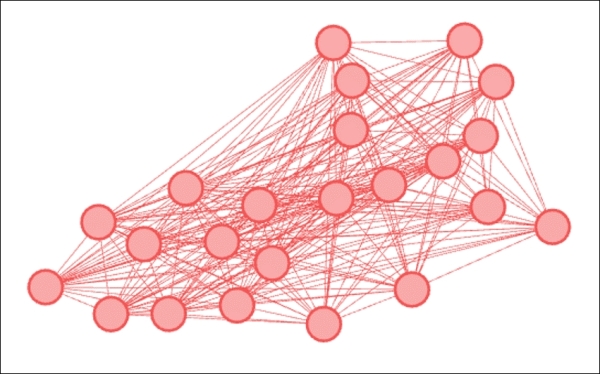
We now have a custom view that shows only nodes from Modularity Class 2, with a Hub value of greater than 0.005, and with edge embeddedness levels greater than 50. Here's our result:
Intersection of node and edge filters
These examples scratched the surface of what can be done by filtering using statistical measures. There are many other conditions and combinations which you can apply to your own networks, perhaps using these instances as templates for knowing how to proceed. While we noted that filtering on these attributes is not always easy or intuitive, I believe you will come to appreciate the power that statistics and filters deliver to your own network analysis.