
The EM algorithm is a generic framework that can be employed in the optimization of many generative models. It was originally proposed in Maximum likelihood from incomplete data via the em algorithm, Dempster A. P., Laird N. M., Rubin D. B., Journal of the Royal Statistical Society, B, 39(1):1–38, 11/1977, where the authors also proved its convergence at different levels of genericity.
For our purposes, we are going to consider a dataset, X, and a set of latent variables, Z, that we cannot observe. They can be part of the original model or introduced artificially as a trick to simplify the problem. A generative model parameterized with the vector θ has a log-likelihood equal to the following:

Of course, a large log-likelihood implies that the model is able to generate the original distribution with a small error. Therefore, our goal is to find the optimal set of parameters θ that maximizes the marginalized log-likelihood (we need to sum—or integrate out for continuous variables—the latent variables out because we cannot observe them):

Theoretically, this operation is correct, but, unfortunately, it's almost always impracticable because of its complexity (in particular, the logarithm of a sum is often very problematic to manage). However, the presence of the latent variables can help us in finding a good proxy that is easy to compute and whose maximization corresponds to the maximization of the original log-likelihood. Let's start by rewriting the expression of the likelihood using the chain rule:

If we consider an iterative process, our goal is to find a procedure that satisfies the following condition:

We can start by considering a generic step:

The first problem to solve is the logarithm of the sum. Fortunately, we can employ the Jensen's inequality, which allows us to move the logarithm inside the summation. Let's first define the concept of a convex function: a function, f(x), defined on a convex set, D, is said to be convex if the following applies:

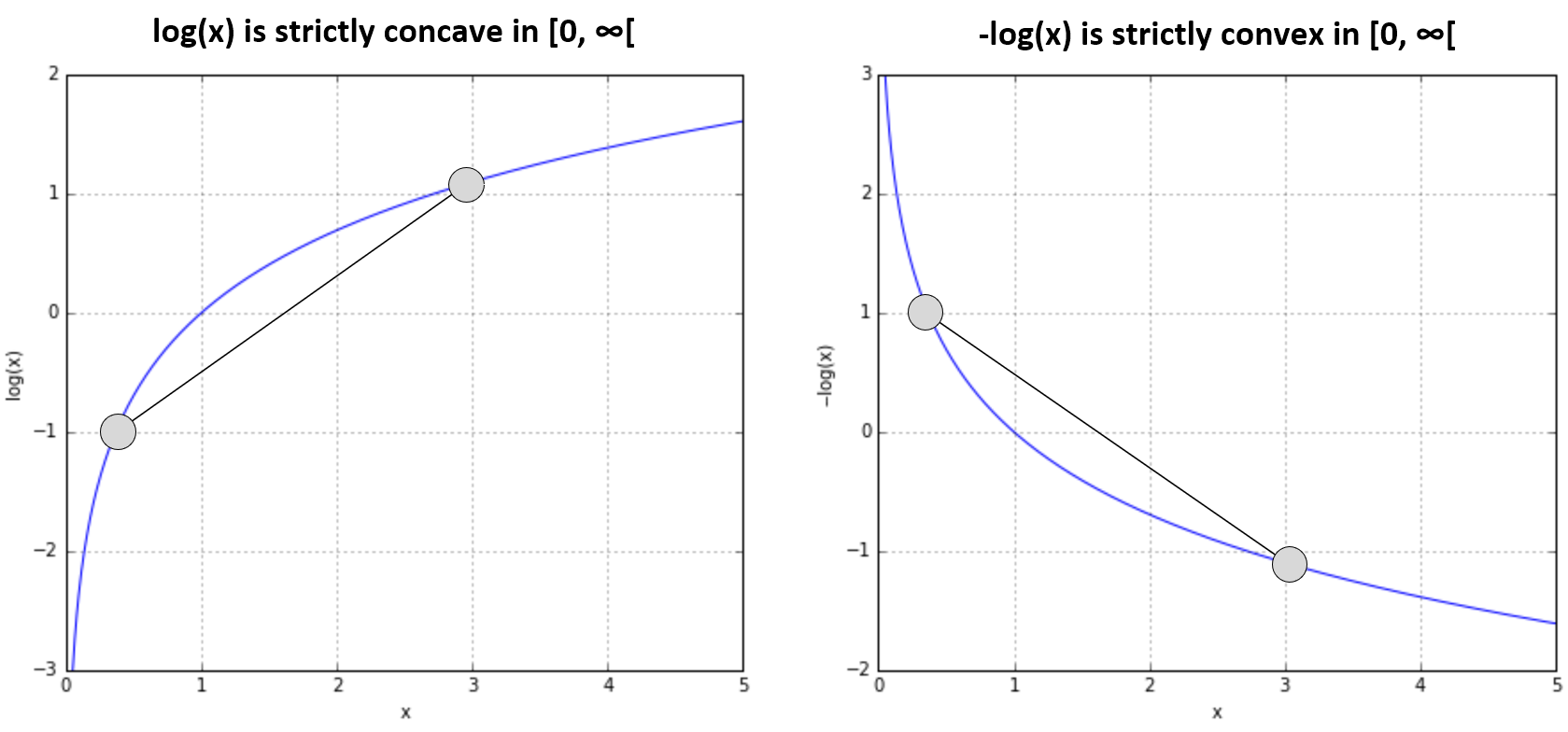
If the inequality is strict, the function is said to be strictly convex. Intuitively, and considering a function of a single variable f(x), the previous definition states that the function is never above the segment that connects two points (x1, f(x1)) and (x2, f(x2)). In the case of strict convexity, f(x) is always below the segment. Inverting these definitions, we obtain the conditions for a function to be concave or strictly concave.
If a function f(x) is concave in D, the function -f(x) is convex in D; therefore, as log(x) is concave in [0, ∞) (or with an equivalent notation in [0, ∞[), -log(x) is convex in [0, ∞), as shown in the following diagram:
The Jensen's inequality (the proof is omitted but further details can be found in Jensen's Operator Inequality, Hansen F., Pedersen G. K., arXiv:math/0204049 [math.OA] states that if f(x) is a convex function defined on a convex set D, if we select n points x1, x2, ..., xn ∈ D and n constants λ1, λ2, ..., λn ≥ 0 satisfying the condition λ1 + λ2 + ... + λn = 1, then the following applies:

Therefore, considering that -log(x) is convex, the Jensen's inequality for log(x) becomes as follows:

Hence, the generic iterative step can be rewritten, as follows:

Applying the Jensen's inequality, we obtain the following:

All the conditions are met, because the terms P(zi|X, θt) are, by definition, bounded between [0, 1] and the sum over all z must always be equal to 1 (laws of probability). The previous expression implies that the following is true:

Therefore, if we maximize the right side of the inequality, we also maximize the log-likelihood. However, the problem can be further simplified, considering that we are optimizing only the parameter vector θ and we can remove all the terms that don't depend on it. Hence, we can define a Q function (there are no relationships with the Q-Learning that we're going to discuss in Chapter 14, Introduction to Reinforcement Learning) whose expression is as follows:

Q is the expected value of the log-likelihood considering the complete data Y = (X, Z) and the current iteration parameter set θt. At each iteration, Q is computed considering the current estimation θt and it's maximized considering the variable θ. It's now clearer why the latent variables can be often artificially introduced: they allow us to apply the Jensen's inequality and transform the original expression into an expected value that is easy to evaluate and optimize.
At this point, we can formalize the EM algorithm:
- Set a threshold Thr (for example, Thr = 0.01)
- Set a random parameter vector θ0.
- While |L(θt|X, Z) - L(θt-1|X, Z)| > Thr:
- E-Step: Compute the Q(θ|θt). In general, this step consists in computing the conditional probability p(z|X, θt) or some of its moments (sometimes, the sufficient statistics are limited to mean and covariance) using the current parameter estimation θt.
- M-Step: Find θt+1 = argmaxθ Q(θ|θt). The new parameter estimation is computed to maximize the Q function.
The procedure ends when the log-likelihood stops increasing or after a fixed number of iterations.