Perceptron was the name that Frank Rosenblatt gave to the first neural model in 1957. A perceptron is a neural network with a single layer of input linear neurons, followed by an output unit based on the sign(•) function (alternatively, it's possible to consider a bipolar unit whose output is -1 and 1). The architecture of a perceptron is shown in the following diagram:

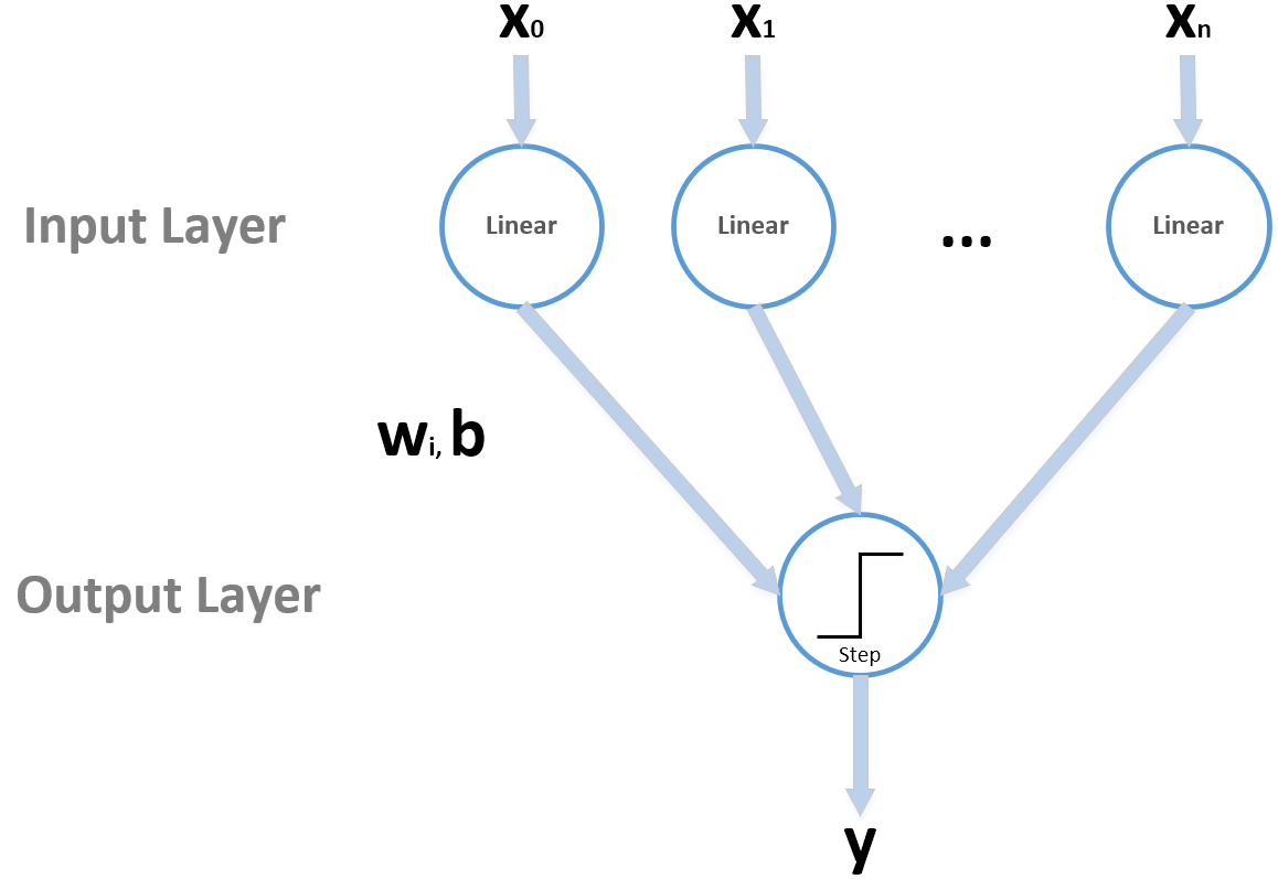
Even if the diagram can appear as quite complex, a perceptron can be summarized by the following equation:

All the vectors are conventionally column-vectors; therefore, the dot product w^Tx_i transforms the input into a scalar, then the bias is added, and the binary output is obtained using the step function, which outputs 1 when z > 0 and 0 otherwise. At this point, a reader could object that the step function is non-linear; however, a non-linearity applied to the output layer is only a filtering operation that has no effect on the actual computation. Indeed, the output is already decided by the linear block, while the step function is employed only to impose a binary threshold. Moreover, in this analysis, we are considering only single-value outputs (even if there are multi-class variants) because our goal is to show the dynamics and also the limitations, before moving to more generic architectures that can be used to solve extremely complex problems.

A perceptron can be trained with an online algorithm (even if the dataset is finite) but it's also possible to employ an offline approach that repeats for a fixed number of iterations or until the total error becomes smaller than a predefined threshold. The procedure is based on the squared error loss function (remember that, conventionally, the term loss is applied to single samples, while the term cost refers to the sum/average of every single loss):

When a sample is presented, the output is computed, and if it is wrong, a weight correction is applied (otherwise the step is skipped). For simplicity, we don't consider the bias, as it doesn't affect the procedure. Our goal is to correct the weights so as to minimize the loss. This can be achieved by computing the partial derivatives with respect to w_i:

Let's suppose that w⁽⁰⁾ = (0, 0) (ignoring the bias) and the sample, x = (1, 1), has y = 1. The perceptron misclassifies the sample, because sign(w^Tx) = 0. The partial derivatives are both equal to -1; therefore, if we subtract them from the current weights, we obtain w⁽¹⁾ = (1, 1) and now the sample is correctly classified because sign(w^Tx) = 1. Therefore, including a learning rate η, the weight update rule becomes as follows:

When a sample is misclassified, the weights are corrected proportionally to the difference between actual linear output and true label. This is a variant of a learning rule called the delta rule, which represented the first step toward the most famous training algorithm, employed in almost any supervised deep learning scenario (we're going to discuss it in the next sections). The algorithm has been proven to converge to a stable solution in a finite number of states as the dataset is linearly separable. The formal proof is quite tedious and very technical, but the reader who is interested can find it in Perceptrons, Minsky M. L., Papert S. A., The MIT Press.

In this chapter, the role of the learning rate becomes more and more important, in particular when the update is performed after the evaluation of a single sample (like in a perceptron) or a small batch. In this case, a high learning rate (that is, one greater than 1.0) can cause an instability in the convergence process because of the magnitude of the single corrections. When working with neural networks, it's preferable to use a small learning rate and repeat the training session for a fixed number of epochs. In this way, the single corrections are limited, and only if they are confirmed by the majority of samples/batches, they can become stable, driving the network to converge to an optimal solution. If, instead, the correction is the consequence of an outlier, a small learning rate can limit its action, avoiding destabilizing the whole network only for a few noisy samples. We are going to discuss this problem in the next sections.

Now, we can describe the full perceptron algorithm and close the paragraph with some important considerations:

1. Select a value for the learning rate η (such as 0.1).
2. Append a constant column (set to 1.0) to the sample vector X. Therefore X_b ∈ ℜ^{M × (n+1)}.
3. Initialize the weight vector w ∈ ℜⁿ⁺¹ with random values sampled from a normal distribution with a small variance (such as 0.05).
4. Set an error threshold Thr (such as 0.0001).
5. Set a maximum number of iterations N_i.
6. Set i = 0.
7. Set e = 1.0.

8. While i < N_i and e > Thr:
   1. Set e = 0.0.
   2. For k=1 to M:
      1. Compute the linear output l_k = w^Tx_k and the threshold one t_k = sign(l_k).
      2. If t_k != y_k:
         1. Compute Δw_j = η(l_k - y_k)x_k^(j).
         2. Update the weight vector.
      3. Set e += (l_k - y_k)² (alternatively it's possible to use the absolute value |l_k - y_k|).
   3. Set e /= M.

The algorithm is very simple, and the reader should have noticed an analogy with a logistic regression. Indeed, this method is based on a structure that can be considered as a perceptron with a sigmoid output activation function (that outputs a real value that can be considered as a probability). The main difference is the training strategy—in a logistic regression, the correction is performed after the evaluation of a cost function based on the negative log likelihood:

This cost function is the well-known cross-entropy and, in the first chapter, we showed that minimizing it is equivalent to reducing the Kullback-Leibler divergence between the true and predicted distribution. In almost all deep learning classification tasks, we are going to employ it, thanks to its robustness and convexity (this is a convergence guarantee in a logistic regression, but unfortunately the property is normally lost in more complex architectures).