
Once the gradients have been computed, the cost function can be moved in the direction of its minimum. However, in practice, it is better to perform an update after the evaluation of a fixed number of training samples (batch). Indeed, the algorithms that are normally employed don't compute the global cost for the whole dataset, because this operation could be very computationally expensive. An approximation is obtained with partial steps, limited to the experience accumulated with the evaluation of a small subset. According to some literature, the expression stochastic gradient descent (SGD) should be used only when the update is performed after every single sample. When this operation is carried out on every k sample, the algorithm is also known as mini-batch gradient descent; however, conventionally SGD is referred to all batches containing k ≥ 1 samples, and we are going to use this expression from now on.
The process can be expressed considering a partial cost function computed using a batch containing k samples:

The algorithm performs a gradient descent by updating the weights according to the following rule:

If we start from an initial configuration θstart, the stochastic gradient descent process can be imagined like the path shown in the following diagram:
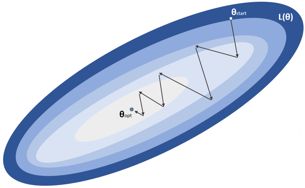
The weights are moved towards the minimum θopt, with many subsequent corrections that could also be wrong considering the whole dataset. For this reason, the process must be repeated several times (epochs), until the validation accuracy reaches its maximum. In a perfect scenario, with a convex cost function L, this simple procedure converges to the optimal configuration. Unfortunately, a deep network is a very complex and non-convex function where plateaus and saddle points are quite common (see Chapter 1, Machine Learning Models Fundamentals). In such a scenario, a vanilla SGD wouldn't be able to find the global optimum and, in many cases, could not even find a close point. For example, in flat regions, the gradients can become so small (also considering the numerical imprecisions) as to slow down the training process until no change is possible (so θ(t+1) ≈ θ(t)). In the next section, we are going to present some common and powerful algorithms that have been developed to mitigate this problem and dramatically accelerate the convergence of deep models.
Before moving on, it's important to mark two important elements. The first one concerns the learning rate, η. This hyperparameter plays a fundamental role in the learning process. As also shown in the figure, the algorithm proceeds jumping from a point to another one (which is not necessarily closer to the optimum). Together with the optimization algorithms, it's absolutely important to correctly tune up the learning rate. A high value (such as 1.0) could move the weights too rapidly increasing the instability. In particular, if a batch contains a few outliers (or simply non-dominant samples), a large η will consider them as representative elements, correcting the weights so to minimize the error. However, subsequent batches could better represent the data generating process, and, therefore, the algorithm must partially revert its modifications in order to compensate the wrong update. For this reason, the learning rate is usually quite small with common values bounded between 0.0001 and 0.01 (in some particular cases, η = 0.1 can be also a valid choice). On the other side, a very small learning rate leads to minimum corrections, slowing down the training process. A good trade-off, which is often the best practice, is to let the learning rate decay as a function of the epoch. In the beginning, η can be higher, because the probability to be close to the optimum is almost null; so, larger jumps can be easily adjusted. While the training process goes on, the weights are progressively moved towards their final configuration and, hence, the corrections become smaller and smaller. In this case, large jumps should be avoided, preferring a fine-tuning. That's why the learning rate is decayed. Common techniques include the exponential decay or a linear one. In both cases, the initial and final values must be chosen according to the specific problem (testing different configurations) and the optimization algorithm. In many cases, the ratio between the start and end value is about 10 or even larger.
Another important hyperparameter is the batch size. There are no silver bullets that allow us to automatically make the right choice, but some considerations can be made. As SGD is an approximate algorithm, larger batches drive to corrections that are probably more similar to the ones obtained considering the whole dataset. However, when the number of samples is extremely high, we don't expect the deep model to map them with a one-to-one association, but instead our efforts are directed to improving the generalization ability. This feature can be re-expressed saying that the network must learn a smaller number of abstractions and reuse them in order to classify new samples. A batch, if sampled correctly, contains a part of these abstract elements and part of the corrections automatically improve the evaluation of a subsequent batch. You can imagine a waterfall process, where a new training step never starts from scratch. However, the algorithm is also called mini-batch gradient descent, because the usual batch size normally ranges from 16 to 512 (larger sizes are uncommon, but always possible), which are values smaller than the number of total samples (in particular in deep learning contexts). A reasonable default value could be 32 samples, but I always invite the reader to test larger values, comparing the performances in terms of training speed and final accuracy.