We want to apply the policy iteration algorithm in order to find an optimal policy for the tunnel environment. Let's start by defining a random initial policy and a value matrix with all values (except the terminal states) equal to 0:

import numpy as np

nb_actions = 4

policy = np.random.randint(0, nb_actions, size=(height, width)).astype(np.uint8)
tunnel_values = np.zeros(shape=(height, width))

The initial random policy (t=0) is shown in the following chart:

The states denoted with ⊗ represent the wells, while the final positive one is represented by the capital letter E. Hence, the initial value matrix (t=0) is:

At this point, we need to define the functions to perform the policy evaluation and improvement steps. As the environment is deterministic, the processes are slightly simpler because the generic transition probability, T(s_i, s_j; a_k), is equal to 1 for the only possible successor and 0 otherwise. In the same way, the policy is deterministic and only a single action is taken into account. The policy evaluation step is performed, freezing the current values and updating the whole matrix, V^(t+1), with V^(t); however, it's also possible to use the new values immediately. I invite the reader to test both strategies in order to find the fastest way. In this example, we are employing a discount factor, γ = 0.9 (it goes without saying that an interesting exercise consists of testing different values and comparing the result of the evaluation process and the final behavior):

import numpy as np

gamma = 0.9

def policy_evaluation():
    old_tunnel_values = tunnel_values.copy() 
    
    for i in range(height):
        for j in range(width): 
            action = policy[i, j]
            
            if action == 0:
                if i == 0:
                    x = 0
                else:
                    x = i - 1
                y = j
                
            elif action == 1:
                if j == width - 1:
                    y = width - 1
                else:
                    y = j + 1
                x = i
                
            elif action == 2:
                if i == height - 1:
                    x = height - 1
                else:
                    x = i + 1
                y = j
                
            else:
                if j == 0:
                    y = 0
                else:
                    y = j - 1
                x = i
                
            reward = tunnel_rewards[x, y]
            tunnel_values[i, j] = reward + (gamma * old_tunnel_values[x, y])

def is_final(x, y):
    if (x, y) in zip(x_wells, y_wells) or (x, y) == (x_final, y_final):
        return True
    return False

def policy_improvement():
    for i in range(height):
        for j in range(width):
            if is_final(i, j):
                continue
            
            values = np.zeros(shape=(nb_actions, ))
            
            values[0] = (tunnel_rewards[i - 1, j] + (gamma * tunnel_values[i - 1, j])) if i > 0 else -np.inf
            values[1] = (tunnel_rewards[i, j + 1] + (gamma * tunnel_values[i, j + 1])) if j < width - 1 else -np.inf
            values[2] = (tunnel_rewards[i + 1, j] + (gamma * tunnel_values[i + 1, j])) if i < height - 1 else -np.inf
            values[3] = (tunnel_rewards[i, j - 1] + (gamma * tunnel_values[i, j - 1])) if j > 0 else -np.inf
            
            policy[i, j] = np.argmax(values).astype(np.uint8)

Once the functions have been defined, we start the policy iteration cycle (with a maximum number of epochs, N_iter = 100,000, and a tolerance threshold equal to 10^-5):

import numpy as np

nb_max_epochs = 100000
tolerance = 1e-5

e = 0

while e < nb_max_epochs:
    e += 1
    old_tunnel_values = tunnel_values.copy()
    policy_evaluation()
    
    if np.mean(np.abs(tunnel_values - old_tunnel_values)) < tolerance:
        old_policy = policy.copy()
        policy_improvement()

        if np.sum(policy - old_policy) == 0:
            break

At the end of the process (in this case, the algorithm converged after 182 iterations, but this value can change with different initial policies), the value matrix is:

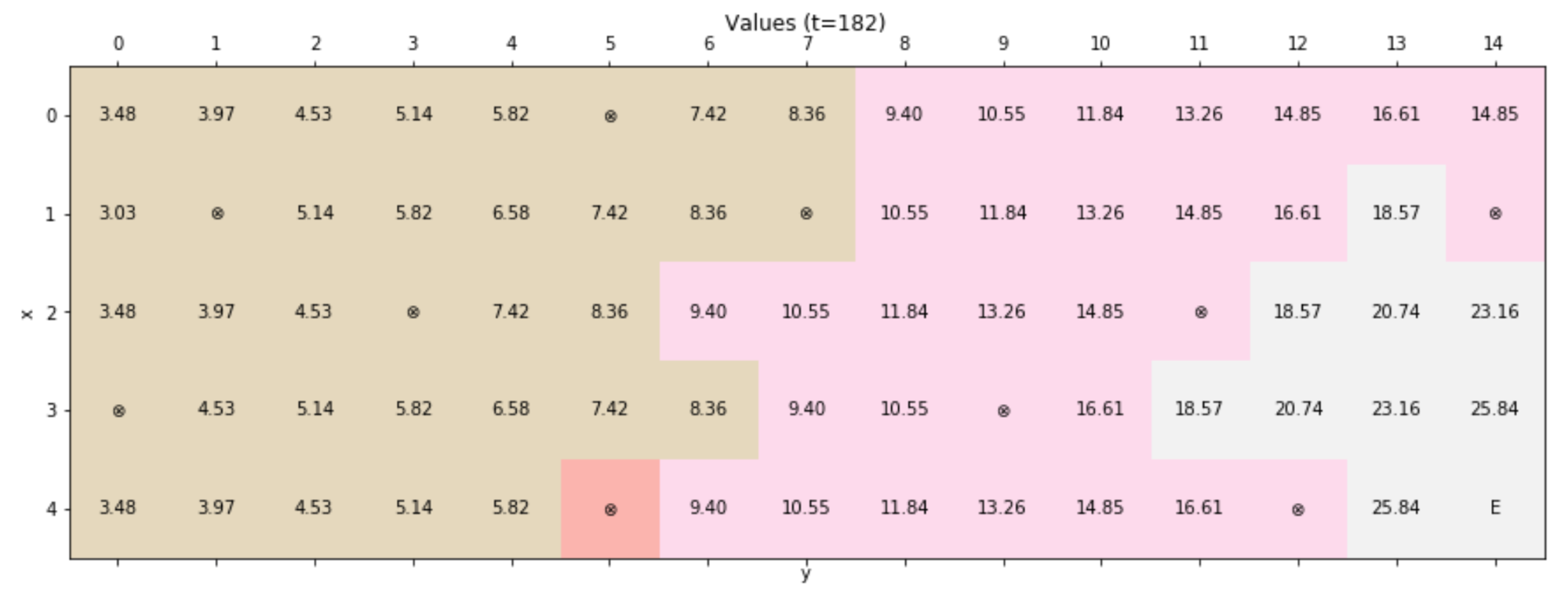
Analyzing the values, it's possible to see how the algorithm discovered that they are an implicit function of the distance between a cell and the ending state. Moreover, the policy always avoids the wells because the maximum value is always found in an adjacent state. It's easy to verify this behavior by plotting the final policy:

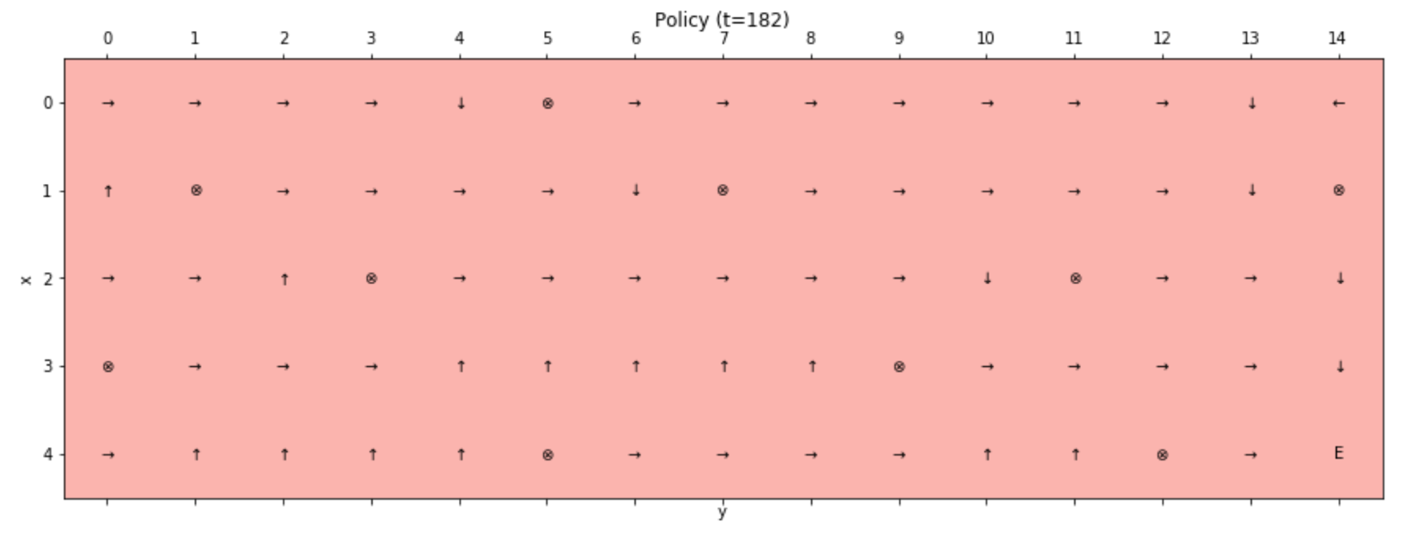
Picking a random initial state, the agent will always reach the ending one, avoiding the wells and confirming the optimality of the policy iteration algorithm.