A valid method to detect the problem of wrongly selected test sets is provided by the cross-validation technique. In particular, we're going to use the K-Fold cross-validation approach. The idea is to split the whole dataset X into a moving test set and a training set (the remaining part). The size of the test set is determined by the number of folds so that, during k iterations, the test set covers the whole original dataset.

In the following diagram, we see a schematic representation of the process:

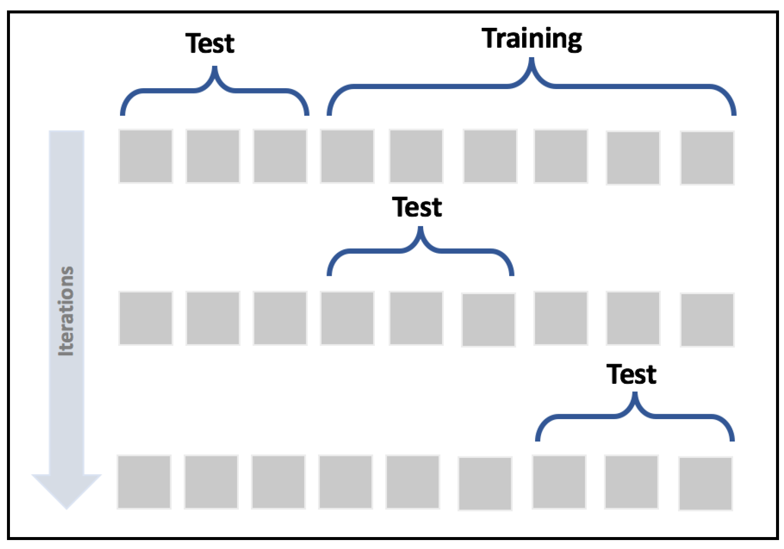
In this way, it's possible to assess the accuracy of the model using different sampling splits, and the training process can be performed on larger datasets; in particular, on (k-1)*N samples. In an ideal scenario, the accuracy should be very similar in all iterations; but in most real cases, the accuracy is quite below average. This means that the training set has been built excluding samples that contain features necessary to let the model fit the separating hypersurface considering the real p_data. We're going to discuss these problems later in this chapter; however, if the standard deviation of the accuracies is too high (a threshold must be set according to the nature of the problem/model), that probably means that X hasn't been drawn uniformly from p_data, and it's useful to evaluate the impact of the outliers in a preprocessing stage. In the following graph, we see the plot of a 15-fold cross-validation performed on a logistic regression:

The values oscillate from 0.84 to 0.95, with an average (solid horizontal line) of 0.91. In this particular case, considering the initial purpose was to use a linear classifier, we can say that all folds yield high accuracies, confirming that the dataset is linearly separable; however, there are some samples (excluded in the ninth fold) that are necessary to achieve a minimum accuracy of about 0.88. 

K-Fold cross-validation has different variants that can be employed to solve specific problems:

• Stratified K-Fold: A Standard K-Fold approach splits the dataset without considering the probability distribution p(y|x), therefore some folds may theoretically contain only a limited number of labels. Stratified K-Fold, instead, tries to split X so that all the labels are equally represented.

• Leave-one-out (LOO): This approach is the most drastic because it creates N folds, each of them containing N-1 training samples and only 1 test sample. In this way, the maximum possible number of samples is used for training, and it's quite easy to detect whether the algorithm is able to learn with sufficient accuracy, or if it's better to adopt another strategy. The main drawback of this method is that N models must be trained, and when N is very large this can cause a performance issue. Moreover, with a large number of samples, the probability that two random values are similar increases, therefore many folds will yield almost identical results. At the same time, LOO limits the possibilities for assessing the generalization ability, because a single test sample is not enough for a reasonable estimation.
• Leave-P-out (LPO): In this case, the number of test samples is set to p (non-disjoint sets), so the number of folds is equal to the binomial coefficient of n over p. This approach mitigates LOO's drawbacks, and it's a trade-off between K-Fold and LOO. The number of folds can be very high, but it's possible to control it by adjusting the number p of test samples; however, if p isn't small or big enough, the binomial coefficient can explode. In fact, when p has about n/2 samples, the number of folds is maximal:

Scikit-Learn implements all those methods (with some other variations), but I suggest always using the cross_val_score() function, which is a helper that allows applying the different methods to a specific problem. In the following snippet based on a polynomial Support Vector Machine (SVM) and the MNIST digits dataset, the function is applied specifying the number of folds (parameter cv). In this way, Scikit-Learn will automatically use Stratified K-Fold for categorical classifications, and Standard K-Fold for all other cases:

from sklearn.datasets import load_digits
from sklearn.model_selection import cross_val_score
from sklearn.svm import SVC

data = load_digits()
svm = SVC(kernel='poly')

skf_scores = cross_val_score(svm, data['data'], data['target'], cv=10)

print(skf_scores)
[ 0.96216216  1.          0.93922652  0.99444444  0.98882682  0.98882682
  0.99441341  0.99438202  0.96045198  0.96590909]

print(skf_scores.mean())
0.978864325583

The accuracy is very high (> 0.9) in every fold, therefore we expect to have even higher accuracy using the LOO method. As we have 1,797 samples, we expect the same number of accuracies:

from sklearn.model_selection import cross_val_score, LeaveOneOut

loo_scores = cross_val_score(svm, data['data'], data['target'], cv=LeaveOneOut())

print(loo_scores[0:100])
[ 1.  1.  1.  1.  1.  0.  1.  1.  1.  1.  1.  1.  1.  1.  1.  1.  1.  1.
  1.  1.  1.  1.  1.  1.  1.  1.  1.  1.  1.  1.  1.  1.  1.  1.  1.  1.
  1.  0.  1.  1.  1.  1.  1.  1.  1.  1.  1.  1.  1.  1.  1.  1.  1.  1.
  1.  1.  1.  1.  1.  1.  1.  1.  1.  1.  1.  1.  1.  1.  1.  0.  1.  1.
  1.  1.  1.  1.  1.  1.  1.  1.  1.  1.  1.  1.  1.  1.  1.  1.  1.  1.
  1.  1.  1.  1.  1.  1.  1.  1.  1.  1.]

print(loo_scores.mean())
0.988870339455

As expected, the average score is very high, but there are still samples that are misclassified. As we're going to discuss, this situation could be a potential candidate for overfitting, meaning that the model is learning perfectly how to map the training set, but it's losing its ability to generalize; however, LOO is not a good method to measure this model ability, due to the size of the validation set.

We can now evaluate our algorithm with the LPO technique. Considering what was explained before, we have selected the smaller Iris dataset and a classification based on a logistic regression. As there are N=150 samples, choosing p = 3, we get 551,300 folds:

from sklearn.datasets import load_iris
from sklearn.linear_model import LogisticRegression
from sklearn.model_selection import cross_val_score, LeavePOut

data = load_iris()

p = 3
lr = LogisticRegression()

lpo_scores = cross_val_score(lr, data['data'], data['target'], cv=LeavePOut(p))

print(lpo_scores[0:100])
[ 1.          1.          1.          1.          1.          1.          1.
  1.          1.          1.          1.          1.          1.          1.
  1.          1.          1.          1.          1.          1.          1.
  1.          1.          1.          1.          1.          1.          1.
  1.          1.          1.          1.          1.          1.          1.
  1.          1.          1.          1.          1.          1.          1.
  1.          1.          1.          1.          1.          1.          1.
  1.          1.          1.          1.          1.          1.          1.
  1.          1.          1.          1.          1.          1.          1.
  1.          0.66666667  ...

print(lpo_scores.mean())
0.955668420098

As in the previous example, we have printed only the first 100 accuracies; however, the global trend can be immediately understood with only a few values.

The cross-validation technique is a powerful tool that is particularly useful when the performance cost is not too high. Unfortunately, it's not the best choice for deep learning models, where the datasets are very large and the training processes can take even days to complete. However, as we're going to discuss, in those cases the right choice (the split percentage), together with an accurate analysis of the datasets and the employment of techniques such as normalization and regularization, allows fitting models that show an excellent generalization ability.