At the beginning of this chapter, we discussed the concept of generic target function so as to optimize in order to solve a machine learning problem. More formally, in a supervised scenario, where we have finite datasets X and Y:

We can define the generic loss function for a single sample as:

J is a function of the whole parameter set, and must be proportional to the error between the true label and the predicted. Another important property is convexity. In many real cases, this is an almost impossible condition; however, it's always useful to look for convex loss functions, because they can be easily optimized through the gradient descent method. We're going to discuss this topic in Chapter 9, Neural Networks for Machine Learning. However, for now, it's useful to consider a loss function as an intermediate between our training process and a pure mathematical optimization. The missing link is the complete data. As already discussed, X is drawn from p_data, so it should represent the true distribution. Therefore, when minimizing the loss function, we're considering a potential subset of points, and never the whole real dataset. In many cases, this isn't a limitation, because, if the bias is null and the variance is small enough, the resulting model will show a good generalization ability (high training and validation accuracy); however, considering the data generating process, it's useful to introduce another measure called expected risk:

This value can be interpreted as an average of the loss function over all possible samples drawn from p_data. Minimizing the expected risk implies the maximization of the global accuracy. When working with a finite number of training samples, instead, it's common to define a cost function (often called a loss function as well, and not to be confused with the log-likelihood):

This is the actual function that we're going to minimize and, divided by the number of samples (a factor that doesn't have any impact), it's also called empirical risk, because it's an approximation (based on real data) of the expected risk. In other words, we want to find a set of parameters so that:

When the cost function has more than two parameters, it's very difficult and perhaps even impossible to understand its internal structure; however, we can analyze some potential conditions using a bidimensional diagram:

The different situations we can observe are:

• The starting point, where the cost function is usually very high due to the error.
• Local minima, where the gradient is null (and the second derivative is positive). They are candidates for the optimal parameter set, but unfortunately, if the concavity isn't too deep, an inertial movement or some noise can easily move the point away.
• Ridges (or local maxima), where the gradient is null, and the second derivative is negative. They are unstable points, because a minimum perturbation allows escaping, reaching lower-cost areas.

• Plateaus, or the region where the surface is almost flat and the gradient is close to zero. The only way to escape a plateau is to keep a residual kinetic energy—we're going to discuss this concept when talking about neural optimization algorithms (Chapter 9, Neural Networks for Machine Learning).
• Global minimum, the point we want to reach to optimize the cost function.

Even if local minima are likely when the number of parameters is small, they become very unlikely when the model has a large number of parameters. In fact, an n-dimensional point θ^* is a local minimum for a convex function (and here, we're assuming L to be convex) only if:

The second condition imposes a positive semi-definite Hessian matrix (equivalently, all principal minors H_n made with the first n rows and n columns must be non-negative), therefore all its eigenvalues λ₀, λ₁, ..., λ_N must be non-negative. This probability decreases with the number of parameters (H is a n×n square matrix and has n eigenvalues), and becomes close to zero in deep learning models where the number of weights can be in the order of 10,000,000 (or even more). The reader interested in a complete mathematical proof can read High Dimensional Spaces, Deep Learning and Adversarial Examples, Dube S., arXiv:1801.00634 [cs.CV]. As a consequence, a more common condition to consider is instead the presence of saddle points, where the eigenvalues have different signs and the orthogonal directional derivatives are null, even if the points are neither local maxima nor minima. Consider, for example, the following plot:

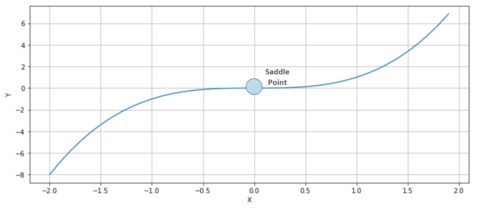
The function is y=x3 whose first and second derivatives are y'=3x2 and y''=6x. Therefore, y'(0)=y''(0)=0. In this case (single-valued function), this point is also called a point of inflection, because at x=0, the function shows a change in the concavity. In three dimensions, it's easier to understand why a saddle point has been called in this way. Consider, for example, the following plot:

The surface is very similar to a horse saddle, and if we project the point on an orthogonal plane, XZ is a minimum, while on another plane (YZ) it is a maximum. Saddle points are quite dangerous, because many simpler optimization algorithms can slow down and even stop, losing the ability to find the right direction. In Chapter 9, Neural Networks for Machine Learning, we're going to discuss some methods that are able to mitigate this kind of problem, allowing deep models to converge.