
In this chapter you’ll learn about the different pitfalls that one should be aware of and that you will encounter while building machine learning systems. You’ll also learn industry standard-efficient designs practiced to solve them.
Throughout this chapter, we’ll mostly be using a dataset from the UCI repository, “Pima Indian diabetes,” which has 768 records, 8 attributes, 2 classes, 268 (34.9%) positive results for diabetes test, and 500 (65.1%) negative results. All patients were females at least 21 years old of Pima Indian heritage.
Attributes of dataset:
Number of times pregnant
Plasma glucose concentration at 2 hours in an oral glucose tolerance test
Diastolic blood pressure (mm Hg)
Triceps skin fold thickness (mm)
2-Hour serum insulin (mu U/ml)
Body mass index (weight in kg/(height in m)^2)
Diabetes pedigree function
Age (years)
Optimal Probability Cutoff Point
Predicted probability is a number between 0 and 1. Traditionally >.5 is the cutoff point used for converting predicted probability to 1 (positive), otherwise it is 0 (negative). This logic works well when your training dataset has equal examples of positive and negative cases; however this is not the case in real-world scenarios.
The solution is to find the optimal cutoff point, that is, the point where the true positive rate is high and the false positive rate is low. Anything above this threshold can be labeled as 1 or else it is 0. Let’s understand this better with an example.
Let’s load the data and check the class distribution. See Listing 4-1.
Listing 4-1. Load data and check the class distribution
import pandas as pdimport pylab as pltimport numpy as npfrom sklearn.cross_validation import train_test_splitfrom sklearn.linear_model import LogisticRegressionfrom sklearn import metrics# read the data indf = pd.read_csv("Data/Diabetes.csv")# target variable % distributionprint df['class'].value_counts(normalize=True)#----output----0 0.6510421 0.348958
Let’s build a quick logistic regression model and check the accuracy. See Listing 4-2.
Listing 4-2. Build logistic regression model and evaluate performance
X = df.ix[:,:8] # independent variablesy = df['class'] # dependent variables# evaluate the model by splitting into train and test setsX_train, X_test, y_train, y_test = train_test_split(X, y, test_size=0.3, random_state=0)# instantiate a logistic regression model, and fitmodel = LogisticRegression()model = model.fit(X_train, y_train)# predict class labels for the train set. The predict fuction converts probability values > .5 to 1 else 0y_pred = model.predict(X_train)# generate class probabilities# Notice that 2 elements will be returned in probs array,# 1st element is probability for negative class,# 2nd element gives probability for positive classprobs = model.predict_proba(X_train)y_pred_prob = probs[:, 1]# generate evaluation metricsprint "Accuracy: ", metrics.accuracy_score(y_train, y_pred)#----output----Accuracy: 0.767225325885
The optimal cutoff would be where the true positive rate (tpr) is high and the false positive rate (fpr) is low, and tpr - (1-fpr) is zero or near to zero. Let’s plot an ROC (receiver operating characteristic) plot of tprvs, 1-fpr. See Listing 4-3.
Listing 4-3. Find optimal cutoff point
# extract false positive, true positive ratefpr, tpr, thresholds = metrics.roc_curve(y_train, y_pred_prob)roc_auc = metrics.auc(fpr, tpr)print("Area under the ROC curve : %f" % roc_auc)i = np.arange(len(tpr)) # index for dfroc = pd.DataFrame({'fpr' : pd.Series(fpr, index=i),'tpr' : pd.Series(tpr, index = i),'1-fpr' : pd.Series(1-fpr, index = i), 'tf' : pd.Series(tpr - (1-fpr), index = i),'thresholds' : pd.Series(thresholds, index = i)})roc.ix[(roc.tf-0).abs().argsort()[:1]]# Plot tpr vs 1-fprfig, ax = plt.subplots()plt.plot(roc['tpr'], label='tpr')plt.plot(roc['1-fpr'], color = 'red', label='1-fpr')plt.legend(loc='best')plt.xlabel('1-False Positive Rate')plt.ylabel('True Positive Rate')plt.title('Receiver operating characteristic')plt.show()#----output----
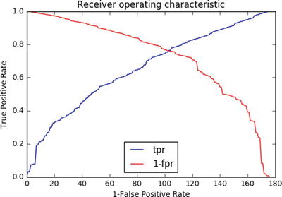
From the chart the point where tpr crosses 1-fpr is the optimal cutoff point. To simplify finding the optimal probability threshold and bringing in reusability, I have made a function to find the optimal probability cutoff point. See Listing 4-4.
Listing 4-4. Function for finding optimal probability cutoff
def Find_Optimal_Cutoff(target, predicted):""" Find the optimal probability cutoff point for a classification model related to event rateParameters----------target : Matrix with dependent or target data, where rows are observationspredicted : Matrix with predicted data, where rows are observationsReturns-------list type, with optimal cutoff value"""fpr, tpr, threshold = metrics.roc_curve(target, predicted)i = np.arange(len(tpr))roc = pd.DataFrame({'tf' : pd.Series(tpr-(1-fpr), index=i), 'threshold' : pd.Series(threshold, index=i)})roc_t = roc.ix[(roc.tf-0).abs().argsort()[:1]]return list(roc_t['threshold'])# Find optimal probability threshold# Note: probs[:, 1] will have probability of being positive labelthreshold = Find_Optimal_Cutoff(y_train, probs[:, 1])print "Optimal Probability Threshold: ", threshold# Applying the threshold to the prediction probabilityy_pred_optimal = np.where(y_pred_prob >= threshold, 1, 0)# Let's compare the accuracy of traditional/normal approach vs optimal cutoffprint " Normal - Accuracy: ", metrics.accuracy_score(y_train, y_pred)print "Optimal Cutoff - Accuracy: ", metrics.accuracy_score(y_train, y_pred_optimal)print " Normal - Confusion Matrix: ", metrics.confusion_matrix(y_train, y_pred)print "Optimal - Cutoff Confusion Matrix: ", metrics.confusion_matrix(y_train, y_pred_optimal)#----output----Optimal Probability Threshold: [0.36133240553264734]Normal - Accuracy: 0.767225325885Optimal Cutoff - Accuracy: 0.761638733706Normal - Confusion Matrix:[[303 40][ 85 109]]Optimal - Cutoff Confusion Matrix:[[261 82][ 46 148]]
Notice that there is no significant difference in overall accuracy between normal vs. optimal cutoff method; both are 76%. However there is a 36% increase in the true positive rate in the optimal cutoff method; that is, you are now able to capture 36% more positive cases as positive; also the false positive (Type I error) has doubled, that is, the probability of predicting an individual not having diabetes as positive has increases.
Which Error Is Costly?
Well, there is no one answer for this question! It depends on the domain, problem that you are trying to address, and the business requirement. In our Pima diabetic case, comparatively a type II error might be more damaging than a type I error, however it’s arguable. See Figure 4-1.
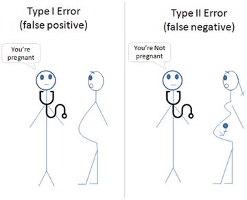
Figure 4-1. Type I vs. Type II error
Rare Event or Imbalanced Dataset
Providing an equal sample of positive and negative instances to the classification algorithm will result in an optimal result. Datasets that are highly skewed toward one or more classes have proven to be a challenge.
Resampling is a common practice to address the imbalanced dataset issue. Although there are many techniques within resampling, here we’ll be learning the three most popular techniques.
Random under-sampling – Reduce majority class to match minority class count.
Random over-sampling – Increase minority class by randomly picking samples within minority class till counts of both class match.
Synthetic Minority Over-Sampling Technique (SMOTE) – Increase minority class by introducing synthetic examples through connecting all k (default = 5) minority class nearest neighbors using feature space similarity (Euclidean distance). See Figure 4-2.
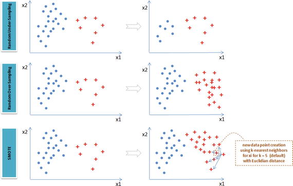
Figure 4-2. Imbalanced dataset handling techniques
Let’s create a sample imbalanced dataset using make_classification function of sklearn. See Listing 4-5.
Listing 4-5. Rare event or imbalanced data handling
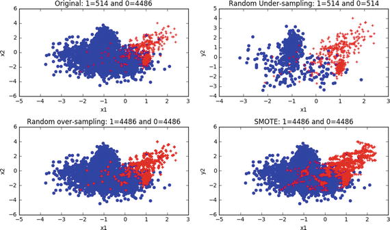
# Load librariesimport matplotlib.pyplot as pltfrom sklearn.datasets import make_classificationfrom imblearn.under_sampling import RandomUnderSamplerfrom imblearn.over_sampling import RandomOverSamplerfrom imblearn.over_sampling import SMOTE# Generate the dataset with 2 features to keep it simpleX, y = make_classification(n_samples=5000, n_features=2, n_informative=2,n_redundant=0, weights=[0.9, 0.1], random_state=2017)print "Positive class: ", y.tolist().count(1)print "Negative class: ", y.tolist().count(0)#----output----Positive class: 514Negative class: 4486
Let’s apply the above described three sampling techniques to the dataset to balance the dataset and visualize for better understanding.
# Apply the random under-samplingrus = RandomUnderSampler()X_RUS, y_RUS = rus.fit_sample(X, y)# Apply the random over-samplingros = RandomOverSampler()X_ROS, y_ROS = ros.fit_sample(X, y)# Apply regular SMOTEsm = SMOTE(kind='regular')X_SMOTE, y_SMOTE = sm.fit_sample(X, y)# Original vs resampled subplotsplt.figure(figsize=(10, 6))plt.subplot(2,2,1)plt.scatter(X[y==0,0], X[y==0,1], marker='o', color='blue')plt.scatter(X[y==1,0], X[y==1,1], marker='+', color='red')plt.xlabel('x1')plt.ylabel('x2')plt.title('Original: 1=%s and 0=%s' %(y.tolist().count(1), y.tolist().count(0)))plt.subplot(2,2,2)plt.scatter(X_RUS[y_RUS==0,0], X_RUS[y_RUS==0,1], marker='o', color='blue')plt.scatter(X_RUS[y_RUS==1,0], X_RUS[y_RUS==1,1], marker='+', color='red')plt.xlabel('x1')plt.ylabel('y2')plt.title('Random Under-sampling: 1=%s and 0=%s' %(y_RUS.tolist().count(1), y_RUS.tolist().count(0)))plt.subplot(2,2,3)plt.scatter(X_ROS[y_ROS==0,0], X_ROS[y_ROS==0,1], marker='o', color='blue')plt.scatter(X_ROS[y_ROS==1,0], X_ROS[y_ROS==1,1], marker='+', color='red')plt.xlabel('x1')plt.ylabel('x2')plt.title('Random over-sampling: 1=%s and 0=%s' %(y_ROS.tolist().count(1), y_ROS.tolist().count(0)))plt.subplot(2,2,4)plt.scatter(X_SMOTE[y_SMOTE==0,0], X_SMOTE[y_SMOTE==0,1], marker='o', color='blue')plt.scatter(X_SMOTE[y_SMOTE==1,0], X_SMOTE[y_SMOTE==1,1], marker='+', color='red')plt.xlabel('x1')plt.ylabel('y2')plt.title('SMOTE: 1=%s and 0=%s' %(y_SMOTE.tolist().count(1), y_SMOTE.tolist().count(0)))plt.tight_layout()plt.show()#----output----
Known Disadvantages
Random Under-Sampling raises the opportunity for loss of information or concepts as we are reducing the majority class.
Random Over-Sampling and SMOTE can lead to over-fitting issues due to multiple related instances.
Which Resampling Technique Is the Best?
Well, yet again there is no one answer to this question! Let’s try a quick classification model on the above three resampled data and compare the accuracy (we’ll use AUC metric as this is one of the best representations of model performance). See Listing 4-6.
Listing 4-6. Build models on various resampling methods and evaluate performance
from sklearn import treefrom sklearn import metricsfrom sklearn.cross_validation import train_test_splitX_RUS_train, X_RUS_test, y_RUS_train, y_RUS_test = train_test_split(X_RUS, y_RUS, test_size=0.3, random_state=2017)X_ROS_train, X_ROS_test, y_ROS_train, y_ROS_test = train_test_split(X_ROS, y_ROS, test_size=0.3, random_state=2017)X_SMOTE_train, X_SMOTE_test, y_SMOTE_train, y_SMOTE_test = train_test_split(X_SMOTE, y_SMOTE, test_size=0.3, random_state=2017)# build a decision tree classifierclf = tree.DecisionTreeClassifier(random_state=2017)clf_rus = clf.fit(X_RUS_train, y_RUS_train)clf_ros = clf.fit(X_ROS_train, y_ROS_train)clf_smote = clf.fit(X_SMOTE_train, y_SMOTE_train)# evaluate model performanceprint " RUS - Train AUC : ",metrics.roc_auc_score(y_RUS_train, clf.predict(X_RUS_train))print "RUS - Test AUC : ",metrics.roc_auc_score(y_RUS_test, clf.predict(X_RUS_test))print "ROS - Train AUC : ",metrics.roc_auc_score(y_ROS_train, clf.predict(X_ROS_train))print "ROS - Test AUC : ",metrics.roc_auc_score(y_ROS_test, clf.predict(X_ROS_test))print " SMOTE - Train AUC : ",metrics.roc_auc_score(y_SMOTE_train, clf.predict(X_SMOTE_train))print "SMOTE - Test AUC : ",metrics.roc_auc_score(y_SMOTE_test, clf.predict(X_SMOTE_test))#----output----RUS - Train AUC : 0.988945248974RUS - Test AUC : 0.983964646465ROS - Train AUC : 0.985666951094ROS - Test AUC : 0.986630288452SMOTE - Train AUC : 1.0SMOTE - Test AUC : 0.956132695918
Here random over-sampling is performing better on both train and test sets. As a best practice, in real-world use cases it is recommended to look at other metrics (such as precision, recall, confusion matrix) and apply business context or domain knowledge to assess the true performance of a model.
Bias and Variance
A fundamental problem with supervised learning is the bias variance trade-off. Ideally a model should have two key characteristics.
Sensitive enough to accurately capture the key patterns in the training dataset.
It should be generalized enough to work well on any unseen datasets.
Unfortunately, while trying to achieve the above-mentioned first point, there is an ample chance of over-fitting to noisy or unrepresentative training data points leading to a failure of generalizing the model. On the other hand, trying to generalize a model may result in failing to capture important regularities.
Bias
If model accuracy is low on a training dataset as well as test dataset the model is said to be under-fitting or that the model has high bias. This means the model is not fitting the training dataset points well in regression or the decision boundary is not separating the classes well in classification; and two key reasons for bias are 1) not including the right features, and 2) not picking the correct order of polynomial degrees for model fitting.
To solve an under-fitting issue or to reduced bias, try including more meaningful features and try to increase the model complexity by trying higher-order polynomial fittings.
Variance
If a model is giving high accuracy on a training dataset, however on a test dataset the accuracy drops drastically, then the model is said to be over-fitting or a model that has high variance. The key reason for over-fitting is using higher-order polynomial degree (may not be required), which will fit decision boundary tools well to all data points including the noise of train dataset, instead of the underlying relationship. This will lead to a high accuracy (actual vs. predicted) in the train dataset and when applied to the test dataset, the prediction error will be high.
To solve the over-fitting issue:
Try to reduce the number of features, that is, keep only the meaningful features or try regularization methods that will keep all the features, however reduce the magnitude of the feature parameter.
Dimension reduction can eliminate noisy features, in turn, reducing the model variance.
Brining more data points to make training dataset large will also reduce variance.
Choosing right model parameters can help to reduce the bias and variance, for example.
Using right regularization parameters can decrease variance in regression-based models.
For a decision tree reducing the depth of the decision tree will reduce the variance. See Figure 4-3.
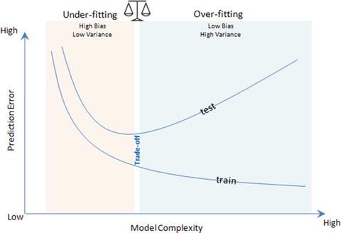
Figure 4-3. Bias Variance trade-off
K-Fold Cross-Validation
K-folds cross-validation splits the training dataset into k-folds without replacement, that is, any given data point will only be part of one of the subset, where k-1 folds are used for the model training and one fold is used for testing. The procedure is repeated k times so that we obtain k models and performance estimates.
We then calculate the average performance of the models based on the individual folds to obtain a performance estimate that is less sensitive to the subpartitioning of the training data compared to the holdout or single fold method. See Figure 4-4.
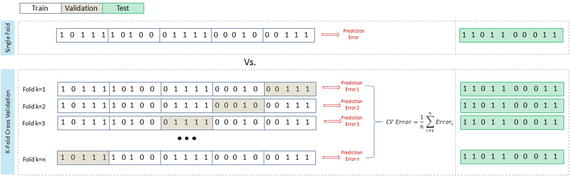
Figure 4-4. K-fold cross-validation
Let’s use K-fold cross-validation of sklearn to build a classification model . See Listing 4-7.
Listing 4-7. K-fold cross-validation
from sklearn.cross_validation import cross_val_score# read the data indf = pd.read_csv("Data/Diabetes.csv")X = df.ix[:,:8].values # independent variablesy = df['class'].values # dependent variables# Normalize Datasc = StandardScaler()sc.fit(X)X = sc.transform(X)# evaluate the model by splitting into train and test setsX_train, X_test, y_train, y_test = train_test_split(X, y, test_size=0.3, random_state=2017)# build a decision tree classifierclf = tree.DecisionTreeClassifier(random_state=2017)# evaluate the model using 10-fold cross-validationtrain_scores = cross_val_score(clf, X_train, y_train, scoring='accuracy', cv=5)test_scores = cross_val_score(clf, X_test, y_test, scoring='accuracy', cv=5)print "Train Fold AUC Scores: ", train_scoresprint "Train CV AUC Score: ", train_scores.mean()print " Test Fold AUC Scores: ", test_scoresprint "Test CV AUC Score: ", test_scores.mean()#---output----Train Fold AUC Scores: [0.80 0.73 0.81 0.76 0.71]Train CV AUC Score: 0.76Test Fold AUC Scores: [0.80 0.78 0.78 0.77 0.8]Test CV AUC Score: 0.79
Stratified K-Fold Cross-Validation
An extended cross-validation is the Stratified K-fold cross-validation, where the class proportions are preserved in each fold, leading to better bias and variance estimates. See Listing 4-8.
Listing 4-8. Stratified k-fold cross-validation
# stratified kfold cross-validationkfold = cross_validation.StratifiedKFold(y=y_train, n_folds=5, random_state=2017)train_scores = []test_scores = []for k, (train, test) in enumerate(kfold):clf.fit(X_train[train], y_train[train])train_score = clf.score(X_train[train], y_train[train])train_scores.append(train_score)# score for test settest_score = clf.score(X_train[test], y_train[test])test_scores.append(test_score)print('Fold: %s, Class dist.: %s, Train Acc: %.3f, Test Acc: %.3f'% (k+1, np.bincount(y_train[train]), train_score, test_score))print(' Train CV accuracy: %.3f' % (np.mean(train_scores)))print('Test CV accuracy: %.3f' % (np.mean(test_scores)))#----output----Fold: 1, Class dist.: [277 152], Train Acc: 0.758, Test Acc: 0.806Fold: 2, Class dist.: [277 152], Train Acc: 0.779, Test Acc: 0.731Fold: 3, Class dist.: [278 152], Train Acc: 0.767, Test Acc: 0.813Fold: 4, Class dist.: [278 152], Train Acc: 0.781, Test Acc: 0.766Fold: 5, Class dist.: [278 152], Train Acc: 0.781, Test Acc: 0.710Train CV accuracy: 0.773Test CV accuracy: 0.765
Ensemble Methods
Ensemble methods enable combining multiple model scores into a single score to create a robust generalized model.
At a high level there are two types of ensemble methods.
Combine multiple models of similar type
Bagging (Bootstrap aggregation)
Boosting
Combine multiple models of various types
Vote Classification
Blending or Stacking
Bagging
Bootstrap aggregation (also known as bagging ) was proposed by Leo Breiman in 1994, which is a model aggregation technique to reduce model variance. The training data is split into multiple samples with replacements called bootstrap samples. Bootstrap sample size will be the same as the original sample size, with 3/4th of the original values and replacement result in repetition of values. See Figure 4-5.
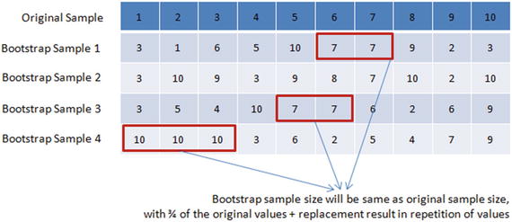
Figure 4-5. Bootstraping
Independent models on each of the bootstrap samples are built, and the average of the predictions for regression or majority vote for classification is used to create the final model.
Figure 4-6 shows the bagging process flow. Let N be the number of bootstrap samples created out of the original training set. For i = 1 to N, train a base machine learning model Ci.
![]()
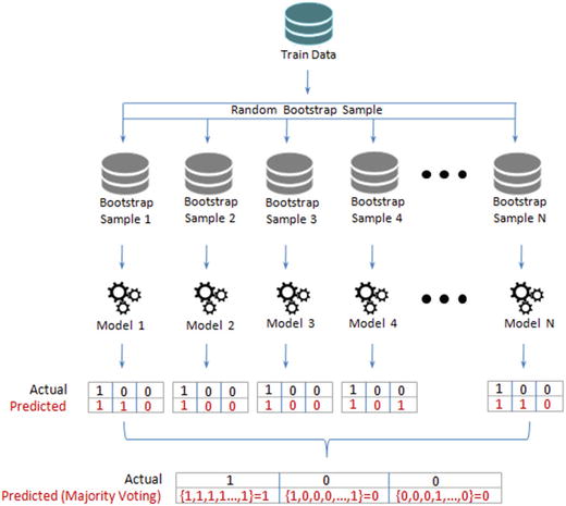
Figure 4-6. Bagging
Let’s compare the performance of a stand-alone decision tree model and a bagging decision tree model of 100 trees. See Listing 4-9.
Listing 4-9. Stand-alone decision tree vs. bagging
# Bagged Decision Trees for Classificationfrom sklearn.ensemble import BaggingClassifierfrom sklearn.tree import DecisionTreeClassifier# read the data indf = pd.read_csv("Data/Diabetes.csv")X = df.ix[:,:8].values # independent variablesy = df['class'].values # dependent variables#NormalizeX = StandardScaler().fit_transform(X)# evaluate the model by splitting into train and test setsX_train, X_test, y_train, y_test = train_test_split(X, y, test_size=0.2, random_state=2017)kfold = cross_validation.StratifiedKFold(y=y_train, n_folds=5, random_state=2017)num_trees = 100# Decision Tree with 5 fold cross validationclf_DT = DecisionTreeClassifier(random_state=2017).fit(X_train,y_train)results = cross_validation.cross_val_score(clf_DT, X_train,y_train, cv=kfold)print "Decision Tree (stand alone) - Train : ", results.mean()print "Decision Tree (stand alone) - Test : ", metrics.accuracy_score(clf_DT.predict(X_test), y_test)# Using Bagging Lets build 100 decision tree models and average/majority vote predictionclf_DT_Bag = BaggingClassifier(base_estimator=clf_DT, n_estimators=num_trees, random_state=2017).fit(X_train,y_train)results = cross_validation.cross_val_score(clf_DT_Bag, X_train, y_train, cv=kfold)print " Decision Tree (Bagging) - Train : ", results.mean()print "Decision Tree (Bagging) - Test : ", metrics.accuracy_score(clf_DT_Bag.predict(X_test), y_test)#----output----Decision Tree (stand alone) - Train : 0.701983077737Decision Tree (stand alone) - Test : 0.753246753247Decision Tree (Bagging) - Train : 0.747461660497Decision Tree (Bagging) - Test : 0.818181818182
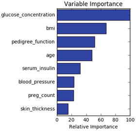
Feature Importance
The decision tree model has an attribute to show important features that are based on the gini or entropy information gain. See Listing 4-10.
Listing 4-10. Decision tree feature importance function
feature_importance = clf_DT.feature_importances_# make importances relative to max importancefeature_importance = 100.0 * (feature_importance / feature_importance.max())sorted_idx = np.argsort(feature_importance)pos = np.arange(sorted_idx.shape[0]) + .5plt.subplot(1, 2, 2)plt.barh(pos, feature_importance[sorted_idx], align='center')plt.yticks(pos, df.columns[sorted_idx])plt.xlabel('Relative Importance')plt.title('Variable Importance')plt.show()#----output----
RandomForest
A subset of observations and a subset of variables are randomly picked to build multiple independent tree-based models. The trees are more un-correlated as only a subset of variables are used during the split of the tree, rather than greedily choosing the best split point in the construction of the tree. See Listing 4-11.
Listing 4-11. RandomForest classifier
from sklearn.ensemble import RandomForestClassifiernum_trees = 100clf_RF = RandomForestClassifier(n_estimators=num_trees).fit(X_train, y_train)results = cross_validation.cross_val_score(clf_RF, X_train, y_train, cv=kfold)print " Random Forest (Bagging) - Train : ", results.mean()print "Random Forest (Bagging) - Test : ", metrics.accuracy_score(clf_RF.predict(X_test), y_test)#----output----Random Forest - Train : 0.758857747224Random Forest - Test : 0.798701298701
Extremely Randomized Trees (ExtraTree)
This algorithm is an effort to introduce more randomness to the bagging process. Tree splits are chosen completely at random from the range of values in the sample at each split, which allows us to reduce the variance of the model further – however, at the cost of a slight increase in bias. See Listing 4-12.
Listing 4-12. Extremely randomized trees (ExtraTree)
from sklearn.ensemble import ExtraTreesClassifiernum_trees = 100clf_ET = ExtraTreesClassifier(n_estimators=num_trees).fit(X_train, y_train)results = cross_validation.cross_val_score(clf_ET, X_train, y_train, cv=kfold)print " ExtraTree - Train : ", results.mean()print "ExtraTree - Test : ", metrics.accuracy_score(clf_ET.predict(X_test), y_test)#----output----ExtraTree - Train : 0.747408778424ExtraTree - Test : 0.811688311688
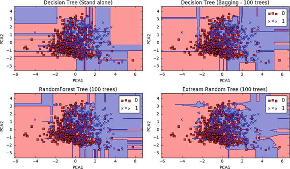
How Does the Decision Boundary Look?
Let’s perform PCA and consider only the first two principal components for easy plotting. The model building code would remain the same as above except that after normalization and before splitting the data to train and test, we will need to add the line below. See Listing 4-13.
Listing 4-13. Plot the decision boundaries
# PCAX = PCA(n_components=2).fit_transform(X)Once we have run the model succesfully we can use the below code to draw decision boundaries for stand alone vs different bagging models.def plot_decision_regions(X, y, classifier):h = .02 # step size in the mesh# setup marker generator and color mapmarkers = ('s', 'x', 'o', '^', 'v')colors = ('red', 'blue', 'lightgreen', 'gray', 'cyan')cmap = ListedColormap(colors[:len(np.unique(y))])# plot the decision surfacex1_min, x1_max = X[:, 0].min() - 1, X[:, 0].max() + 1x2_min, x2_max = X[:, 1].min() - 1, X[:, 1].max() + 1xx1, xx2 = np.meshgrid(np.arange(x1_min, x1_max, h),np.arange(x2_min, x2_max, h))Z = classifier.predict(np.array([xx1.ravel(), xx2.ravel()]).T)Z = Z.reshape(xx1.shape)plt.contourf(xx1, xx2, Z, alpha=0.4, cmap=cmap)plt.xlim(xx1.min(), xx1.max())plt.ylim(xx2.min(), xx2.max())for idx, cl in enumerate(np.unique(y)):plt.scatter(x=X[y == cl, 0], y=X[y == cl, 1],alpha=0.8, c=cmap(idx),marker=markers[idx], label=cl)# Plot the decision boundaryplt.figure(figsize=(10,6))plt.subplot(221)plot_decision_regions(X, y, clf_DT)plt.title('Decision Tree (Stand alone)')plt.xlabel('PCA1')plt.ylabel('PCA2')plt.subplot(222)plot_decision_regions(X, y, clf_DT_Bag)plt.title('Decision Tree (Bagging - 100 trees)')plt.xlabel('PCA1')plt.ylabel('PCA2')plt.legend(loc='best')plt.subplot(223)plot_decision_regions(X, y, clf_RF)plt.title('RandomForest Tree (100 trees)')plt.xlabel('PCA1')plt.ylabel('PCA2')plt.legend(loc='best')plt.subplot(224)plot_decision_regions(X, y, clf_ET)plt.title('Extream Random Tree (100 trees)')plt.xlabel('PCA1')plt.ylabel('PCA2')plt.legend(loc='best')plt.tight_layout()#----output----Decision Tree (stand alone) - Train : 0.595875198308Decision Tree (stand alone) - Test : 0.616883116883Decision Tree (Bagging) - Train : 0.646298254892Decision Tree (Bagging) - Test : 0.714285714286Random Forest - Train : 0.665917503966Random Forest - Test : 0.707792207792ExtraTree - Train : 0.635034373347ExtraTree - Test : 0.707792207792
Bagging – Essential Tuning Parameters
n_estimators: This is the number of trees, the larger the better. Note that beyond a certain point the results will not improve significantly.
max_features: This is the random subset of features to be used for splitting node, the lower the better to reduce variance (but increases bias). Ideally, for a regression problem it should be equal to n_features (total number of features) and for classification square root of n_features.
n_jobs: Number of cores to be used for parallel construction of trees. If set to -1, all available cores in the system are used, or you can specify the number.
Boosting
Freud and Schapire in 1995 introduced the concept of boosting with the well-known AdaBoost algorithm (adaptive boosting). The core concept of boosting is that rather than an independent individual hypothesis, combining hypotheses in a sequential order increases the accuracy. Essentially, boosting algorithms convert the weak learners into strong learners. Boosting algorithms are well designed to address the bias problems.
At a high level the AdaBoosting process can be divided into three steps. See Figure 4-7.
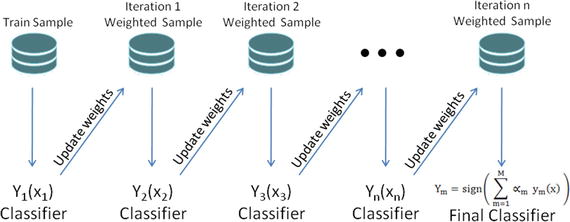
Figure 4-7. AdaBoosting
Assign uniform weights for all data points W0(x) = 1 / N, where N is the total number of training data points.
At each iteration fit a classifier ym(xn) to the training data and update weights to minimize the weighted error function.
The weight is calculated as
 .
.The hypothesis weight or the loss function is given by
 , and the term rate is given by
  , where
The final model is given by
Example Illustration for AdaBoost
Let’s consider a training data with two class labels of 10 data points. Assume, initially all the data points will have equal weights given by, for example, 1/10 as shown in Figure 4-8 below.
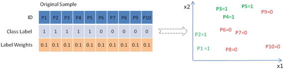
Figure 4-8. Sample dataset with 10 data points
Boosting Iteration 1
Notice in Figure 4-9 that three points of positive class are misclassified by the first simple classification model, so they will be assigned higher weights. The error term and loss function (learning rate) is calcuated as 0.30 and 0.42 respectively. The data points P3, P4, and P5 will get higher weight (0.15) due to misclassification, whereas other data points will retain the original weight (0.1).
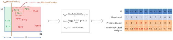
Figure 4-9. Ym1 the first classification or hypothesis
Boosting Iteration 2
Let’s fit another classification model as shown in Figure 4-10 below and notice that three data points of negative class are misclassified. The data points P6, P7, and P8 are misclassified. Hence these will be assigned higher weights of 0.17 as calculated, whereas the remaining data point’s weights will remain the same as they are correctly classified.
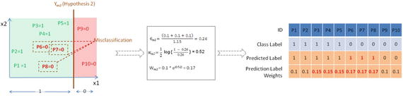
Figure 4-10. Ym2 the second classification or hypothesis
Boosting Iteration 3
The third classification model has misclassified a toal of three data points, that is, two positive class P1, P2, and one negative class P9. So these misclassified data points will be assigned a new higher weight of 0.19 as calculated and the remaining data points will retain their earlier weights. See Figure 4-11.
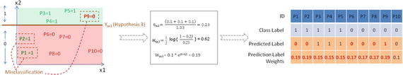
Figure 4-11. Ym3 the third classification or hypothesis
Final Model
Now as per the AdaBoost algorithm, let’s combine the weak classification models as shown in Figure 4-12 below. Notice that the final model combined model will have a minimum error term and maximum learning rate leading to a higher degree of accuracy.
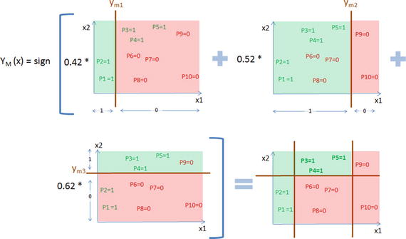
Figure 4-12. AdaBoost algorithm to combine weak classifiers
Let’s pick weak predictors from the Pima diabetic dataset and compare the performance of a stand-alone decision tree model vs. AdaBoost with 100 boosting rounds on the decision tree model. See Listing 4-14.
Listing 4-14. Stand-alone decision tree vs. adaboost
# Bagged Decision Trees for Classificationfrom sklearn.ensemble import AdaBoostClassifierfrom sklearn.tree import DecisionTreeClassifier# read the data indf = pd.read_csv("Data/Diabetes.csv")# Let's use some week features to build the treeX = df[['age','serum_insulin']] # independent variablesy = df['class'].values # dependent variables#NormalizeX = StandardScaler().fit_transform(X)# evaluate the model by splitting into train and test setsX_train, X_test, y_train, y_test = train_test_split(X, y, test_size=0.2, random_state=2017)kfold = cross_validation.StratifiedKFold(y=y_train, n_folds=5, random_state=2017)num_trees = 100# Dection Tree with 5 fold cross validation# lets restrict max_depth to 1 to have more impure leavesclf_DT = DecisionTreeClassifier(max_depth=1, random_state=2017).fit(X_train,y_train)results = cross_validation.cross_val_score(clf_DT, X_train,y_train, cv=kfold)print "Decision Tree (stand alone) - Train : ", results.mean()print "Decision Tree (stand alone) - Test : ", metrics.accuracy_score(clf_DT.predict(X_test), y_test)# Using Adaptive Boosting of 100 iterationclf_DT_Boost = AdaBoostClassifier(base_estimator=clf_DT, n_estimators=num_trees, learning_rate=0.1, random_state=2017).fit(X_train,y_train)results = cross_validation.cross_val_score(clf_DT_Boost, X_train, y_train, cv=kfold)print " Decision Tree (AdaBoosting) - Train : ", results.mean()print "Decision Tree (AdaBoosting) - Test : ", metrics.accuracy_score(clf_DT_Boost.predict(X_test), y_test)#----output----Decision Tree (stand alone) - Train : 0.635113696457Decision Tree (stand alone) - Test : 0.649350649351Decision Tree (AdaBoosting) - Train : 0.688709677419Decision Tree (AdaBoosting) - Test : 0.707792207792Notice that in this case AdaBoost algorithm has given an average rise of 9% in accuracy score between train / test dataset compared to the stanalone decision tree model.
Gradient Boosting
Due to the stage-wise addictivity, the loss function can be represented in a form suitable for optimization. This gave birth to a class of generalized boosting algorithms known as generalized boosting algorithm (GBM). Gradient boosting is an example implementation of GBM and it can work with different loss functions such as regression, classification, risk modeling, etc. As the name suggests it is a boosting algorithm that identifies shortcomings of a weak learner by gradients (AdaBoost uses high-weight data points), hence the name Gradient Boosting. See Listing 4-15.
Iteratively fit a classifier ym(xn) to the training data. The initial model will be with a constant value
Calculate the loss (i.e., the predicted value vs. actual value) for each model fit iteration gm(x)or compute the negative gradient, and use it to fit a new base learner function hm(x), and find the best gradient decent step-size
Update the function estimate
 and output ym(x)
Listing 4-15. Gradient boosting classifier
from sklearn.ensemble import GradientBoostingClassifier# Using Gradient Boosting of 100 iterationsclf_GBT = GradientBoostingClassifier(n_estimators=num_trees, learning_rate=0.1, random_state=2017).fit(X_train, y_train)results = cross_validation.cross_val_score(clf_GBT, X_train, y_train, cv=kfold)print " Gradient Boosting - CV Train : %.2f" % results.mean()print "Gradient Boosting - Train : %.2f" % metrics.accuracy_score(clf_GBT.predict(X_train), y_train)print "Gradient Boosting - Test : %.2f" % metrics.accuracy_score(clf_GBT.predict(X_test), y_test)#----output----Gradient Boosting - CV Train : 0.70Gradient Boosting - Train : 0.81Gradient Boosting - Test : 0.66
Let’s look at the digit classification to illustrate how the model performance improves with each iteration.
from sklearn.ensemble import GradientBoostingClassifierdf= pd.read_csv('Data/digit.csv')X = df.ix[:,1:17].valuesy = df['lettr'].values# evaluate the model by splitting into train and test setsX_train, X_test, y_train, y_test = train_test_split(X, y, test_size=0.2, random_state=2017)kfold = cross_validation.StratifiedKFold(y=y_train, n_folds=5, random_state=2017)num_trees = 10clf_GBT = GradientBoostingClassifier(n_estimators=num_trees, learning_rate=0.1, max_depth=3, random_state=2017).fit(X_train, y_train)results = cross_validation.cross_val_score(clf_GBT, X_train, y_train, cv=kfold)print " Gradient Boosting - Train : ", metrics.accuracy_score(clf_GBT.predict(X_train), y_train)print "Gradient Boosting - Test : ", metrics.accuracy_score(clf_GBT.predict(X_test), y_test)# Let's predict for the letter 'T' and understand how the prediction accuracy changes in each boosting iterationX_valid= (2,8,3,5,1,8,13,0,6,6,10,8,0,8,0,8)print "Predicted letter: ", clf_GBT.predict(X_valid)# Staged prediction will give the predicted probability for each boosting iterationstage_preds = list(clf_GBT.staged_predict_proba(X_valid))final_preds = clf_GBT.predict_proba(X_valid)# Plotx = range(1,27)label = np.unique(df['lettr'])plt.figure(figsize=(10,3))plt.subplot(131)plt.bar(x, stage_preds[0][0], align='center')plt.xticks(x, label)plt.xlabel('Label')plt.ylabel('Prediction Probability')plt.title('Round One')plt.autoscale()plt.subplot(132)plt.bar(x, stage_preds[5][0],align='center')plt.xticks(x, label)plt.xlabel('Label')plt.ylabel('Prediction Probability')plt.title('Round Five')plt.autoscale()plt.subplot(133)plt.bar(x, stage_preds[9][0],align='center')plt.xticks(x, label)plt.autoscale()plt.xlabel('Label')plt.ylabel('Prediction Probability')plt.title('Round Ten')plt.tight_layout()plt.show()#----output----Gradient Boosting - Train : 0.7525625Gradient Boosting - Test : 0.7305Predicted letter: 'T'
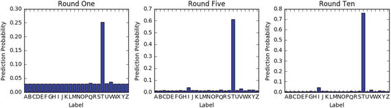
Gradient boosting corrects the erroneous boosting iteration’s negative impact in subsequent iterations. Notice that in the first iteration the predicted probability for letter ‘T’ is 0.25 and it gradually increased to 0.76 by the 10th iteration, whereas the proability percentage for other letters have decreased over each round.
Boosting – Essential Tuning Parameters
Model complexity and over-fitting can be controlled by using correct values for two categories of parameters.
Tree structure
n_estimators: This is the number of weak learners to be built.
max_depth: Maximum depth of the individual estimators. The best value depends on the interaction of the input variables.
min_samples_leaf: This will be helpful to ensure sufficient number of samples result in leaf.
subsample: The fraction of sample to be used for fitting individual models (default=1). Typically .8 (80%) is used to introduce random selection of samples, which, in turn, increases the robustness against over-fitting.
Regularization parameter
learning_rate: this controls the magnitude of change in estimators. Lower learning rate is better, which requires higher n_estimators (that is the trade-off).
Xgboost (eXtreme Gradient Boosting)
In March 2014, Tianqui Chen built xgboost in C++ as part of the Distributed (Deep) Machine Learning Community, and it has an interface for Python. It is an extended, more regularized version of a gradient boosting algorithm. This is one of the most well-performing large-scale, scalable machine learning algorithms that has been playing a major role in winning solutions of Kaggle (forum for predictive modeling and analytics competition) data science competition.
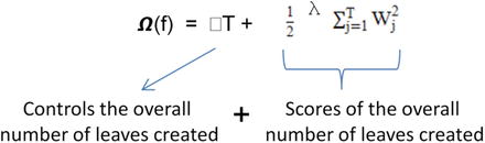
XGBoost objective function obj(ϴ) = 
Regularization term is given by
The gradient descent technique is used for optimizing the objective function, and more mathematics about the algorithms can be found at the following site: http://xgboost.readthedocs.io/en/latest/
Some of the key advantages of the xgboost algorithm are these:
It implements parallel processing.
It has a built-in standard to handle missing values, which means user can specify a particular value different than other observations (such as -1 or -999) and pass it as a parameter.
It will split the tree up to a maximum depth unlike Gradient Boosting where it stops splitting node on encounter of a negative loss in the split.
XGboost has bundle of parameters, and at a high level we can group them into three categories. Let’s look at the most important within these categories.
General Parameters
nthread – Number of parallel threads; if not given a value all cores will be used.
Booster – This is the type of model to be run with gbtree (tree-based model) being the default. ‘gblinear’ to be used for linear models
Boosting Parameters
eta – This is the learning rate or step size shrinkage to prevent over-fitting; default is 0.3 and it can range between 0 to 1
max_depth – Maximum depth of tree with default being 6.
min_child_weight – Minimum sum of weights of all observations required in child. Start with 1/square root of event rate
colsample_bytree – Fraction of columns to be randomly sampled for each tree with default value of 1.
Subsample –Fraction of observations to be randomly sampled for each tree with default of value of 1. Lowering this value makes algorithm conservative to avoid over-fitting.
lambda - L2 regularization term on weights with default value of 1.
alpha - L1 regularization term on weight.
Task Parameters
objective – This defines the loss function to be minimized with default value ‘reg:linear’. For binary classification it should be ‘binary:logistic’ and for multiclass ‘multi:softprob’ to get the probability value and ‘multi:softmax’ to get predicted class. For multiclass num_class (number of unique classes) to be specified.
eval_metric – Metric to be use for validating model performance.
sklearn has a wrapper for xgboost (XGBClassifier). Let’s continue with the diabetic’s dataset and build a model using the weak learner. See Listing 4-16.
Listing 4-16. xgboost classifer using sklearn wrapper
import xgboost as xgbfrom xgboost.sklearn import XGBClassifier# read the data indf = pd.read_csv("Data/Diabetes.csv")# Let's use some weak features as predictorspredictors = ['age','serum_insulin']target = 'class'# Most common preprocessing step include label encoding and missing value treatmentfrom sklearn import preprocessingfor f in df.columns:if df[f].dtype=='object':lbl = preprocessing.LabelEncoder()lbl.fit(list(df[f].values))df[f] = lbl.transform(list(df[f].values))df.fillna((-999), inplace=True) # missing value treatment# Let's use some week features to build the treeX = df[['age','serum_insulin']] # independent variablesy = df['class'].values # dependent variables#NormalizeX = StandardScaler().fit_transform(X)# evaluate the model by splitting into train and test setsX_train, X_test, y_train, y_test = train_test_split(X, y, test_size=0.2, random_state=2017)num_rounds = 100clf_XGB = XGBClassifier(n_estimators = num_rounds,objective= 'binary:logistic',seed=2017)# use early_stopping_rounds to stop the cv when there is no score imporovementclf_XGB.fit(X_train,y_train, early_stopping_rounds=20, eval_set=[(X_test, y_test)], verbose=False)results = cross_validation.cross_val_score(clf_XGB, X_train,y_train, cv=kfold)print " xgBoost - CV Train : %.2f" % results.mean()print "xgBoost - Train : %.2f" % metrics.accuracy_score(clf_XGB.predict(X_train), y_train)print "xgBoost - Test : %.2f" % metrics.accuracy_score(clf_XGB.predict(X_test), y_test)#----output----
Now let’s also look at how to build a model using xgboost native interface. DMatrix the internal data structure of xgboost for input data. It is good practice to convert a large dataset to DMatrix object to save preprocessing time. See Listing 4-17.
Listing 4-17. xgboost using it’s native python package code
xgtrain = xgb.DMatrix(X_train, label=y_train, missing=-999)xgtest = xgb.DMatrix(X_test, label=y_test, missing=-999)# set xgboost paramsparam = {'max_depth': 3, # the maximum depth of each tree'objective': 'binary:logistic'}clf_xgb_cv = xgb.cv(param, xgtrain, num_rounds,stratified=True,nfold=5,early_stopping_rounds=20,seed=2017)print ("Optimal number of trees/estimators is %i" % clf_xgb_cv.shape[0])watchlist = [(xgtest,'test'), (xgtrain,'train')]clf_xgb = xgb.train(param, xgtrain,clf_xgb_cv.shape[0], watchlist)# predict function will produce the probability# so we'll use 0.5 cutoff to convert probability to class labely_train_pred = (clf_xgb.predict(xgtrain, ntree_limit=clf_xgb.best_iteration) > 0.5).astype(int)y_test_pred = (clf_xgb.predict(xgtest, ntree_limit=clf_xgb.best_iteration) > 0.5).astype(int)print "XGB - Train : %.2f" % metrics.accuracy_score(y_train_pred, y_train)print "XGB - Test : %.2f" % metrics.accuracy_score(y_test_pred, y_test)#----output----Optimal number of trees (estimators) is 7[0] test-error:0.344156 train-error:0.299674[1] test-error:0.324675 train-error:0.273616[2] test-error:0.272727 train-error:0.281759[3] test-error:0.266234 train-error:0.278502[4] test-error:0.266234 train-error:0.273616[5] test-error:0.311688 train-error:0.254072[6] test-error:0.318182 train-error:0.254072XGB - Train : 0.75XGB - Test : 0.69
Ensemble Voting – Machine Learning’s Biggest Heroes United
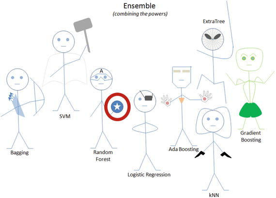
Figure 4-13. Ensemble: ML's biggest heroes united
A voting classifier enables us to combine the predictions through majority voting from multiple machine learning algorithms of different types, unlike Bagging/Boosting where similar types of multiple classifiers are used for majority voting.
First you can create multiple stand-alone models from your training dataset. Then a voting classifier can be used to wrap your models and average the predictions of the sub-models when asked to make predictions for new data. The predictions of the sub-models can be weighted, but specifying the weights for classifiers manually or even heuristically is difficult. More advanced methods can learn how to best weigh the predictions from sub-models, but this is called stacking (stacked aggregation) and is currently not provided in scikit-learn.
Let’s build individual models on the Pima diabetes dataset and try the voting classifier to combine model results to compare the change in accuracy. See Listing 4-18.
Listing 4-18. Ensemble model
import pandas as pdimport numpy as np# set seed for reproducabilitynp.random.seed(2017)import statsmodels.api as smfrom sklearn import metricsfrom sklearn.linear_model import LogisticRegressionfrom sklearn.ensemble import RandomForestClassifierfrom sklearn.svm import SVCfrom sklearn.neighbors import KNeighborsClassifierfrom sklearn.tree import DecisionTreeClassifierfrom sklearn.ensemble import AdaBoostClassifierfrom sklearn.ensemble import BaggingClassifierfrom sklearn.ensemble import GradientBoostingClassifier# currently its available as part of mlxtend and not sklearnfrom mlxtend.classifier import EnsembleVoteClassifierfrom sklearn import cross_validationfrom sklearn import metricsfrom sklearn.cross_validation import train_test_split# read the data indf = pd.read_csv("Data/Diabetes.csv")X = df.ix[:,:8] # independent variablesy = df['class'] # dependent variables# evaluate the model by splitting into train and test setsX_train, X_test, y_train, y_test = train_test_split(X, y, test_size=0.3, random_state=2017)LR = LogisticRegression(random_state=2017)RF = RandomForestClassifier(n_estimators = 100, random_state=2017)SVM = SVC(random_state=0, probability=True)KNC = KNeighborsClassifier()DTC = DecisionTreeClassifier()ABC = AdaBoostClassifier(n_estimators = 100)BC = BaggingClassifier(n_estimators = 100)GBC = GradientBoostingClassifier(n_estimators = 100)clfs = []print('5-fold cross validation: ')for clf, label in zip([LR, RF, SVM, KNC, DTC, ABC, BC, GBC],['Logistic Regression','Random Forest','Support Vector Machine','KNeighbors','Decision Tree','Ada Boost','Bagging','Gradient Boosting']):scores = cross_validation.cross_val_score(clf, X_train, y_train, cv=5, scoring='accuracy')print("Train CV Accuracy: %0.2f (+/- %0.2f) [%s]" % (scores.mean(), scores.std(), label))md = clf.fit(X, y)clfs.append(md)print("Test Accuracy: %0.2f " % (metrics.accuracy_score(clf.predict(X_test), y_test)))#----output----5-fold cross validation:Train CV Accuracy: 0.76 (+/- 0.03) [Logistic Regression]Test Accuracy: 0.79Train CV Accuracy: 0.74 (+/- 0.03) [Random Forest]Test Accuracy: 1.00Train CV Accuracy: 0.65 (+/- 0.00) [Support Vector Machine]Test Accuracy: 1.00Train CV Accuracy: 0.70 (+/- 0.05) [KNeighbors]Test Accuracy: 0.84Train CV Accuracy: 0.69 (+/- 0.02) [Decision Tree]Test Accuracy: 1.00Train CV Accuracy: 0.73 (+/- 0.04) [Ada Boost]Test Accuracy: 0.83Train CV Accuracy: 0.75 (+/- 0.04) [Bagging]Test Accuracy: 1.00Train CV Accuracy: 0.75 (+/- 0.03) [Gradient Boosting]Test Accuracy: 0.92
From the above benchmarking we see that ‘Logistic Regression’, ‘Random Forest’, ‘Bagging’, and Ada/Gradient Boosting algorithms are giving better accuracy compared to other models. Let’s combine non-similar models such as Logistic regression (base model), Random Forest (bagging model), and gradient boosting (boosting model) to create a robust generalized model.
Hard Voting vs. Soft Voting
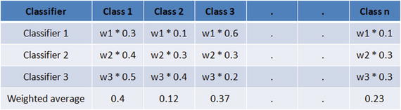
Majority voting is also known as hard voting. The argmax of the sum of predicted probabilities is known as soft voting. Parameter ‘weights’ can be used to assign specific weights to classifiers. The predicted class probabilities for each classifier are multiplied by the classifier weight and averaged. Then the final class label is derived from the highest average probability class label.
Assume we assign equal weight of 1 to all classifiers (see Table 4-1). Based on soft voting, the predicted class label is 1, as it has the highest average probability. See also Listing 4-19.
Table 4-1. Soft voting
Note
Some classifiers of scikit-learn do not support the predict_proba method.
Listing 4-19. Ensemble voting model
# Ensemble Votingclfs = []print('5-fold cross validation: ')ECH = EnsembleVoteClassifier(clfs=[LR, RF, GBC], voting='hard')ECS = EnsembleVoteClassifier(clfs=[LR, RF, GBC], voting='soft', weights=[1,1,1])for clf, label in zip([ECH, ECS],['Ensemble Hard Voting','Ensemble Soft Voting']):scores = cross_validation.cross_val_score(clf, X_train, y_train, cv=5, scoring='accuracy')print("Train CV Accuracy: %0.2f (+/- %0.2f) [%s]" % (scores.mean(), scores.std(), label))md = clf.fit(X, y)clfs.append(md)print("Test Accuracy: %0.2f " % (metrics.accuracy_score(clf.predict(X_test), y_test)))#----output----5-fold cross validation:Train CV Accuracy: 0.75 (+/- 0.02) [Ensemble Hard Voting]Test Accuracy: 0.93Train CV Accuracy: 0.76 (+/- 0.02) [Ensemble Soft Voting]Test Accuracy: 0.95
Stacking
Wolpert David H presented (in 1992) the concept of stacked generalization, most commonly known as ‘stacking’ in his publication with the journal Neural Networks. In stacking initially, you train multiple base models of different types on training/test datasets. It is ideal to mix models that work differently (kNN, bagging, boosting, etc.) so that it can learn some part of the problem. At level 1, use the predicted values from base models as features and train a model that is known as a meta-model, thus combining the learning of an individual model will result in improved accuracy. This is a simple level 1 stacking, and similarly you can stack multiple levels of different type of models. See Figure 4-14.
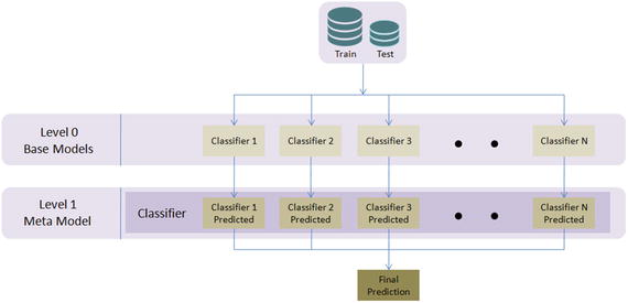
Figure 4-14. Simple Level 2 stacking model
Let’s apply the stacking concept discussed above on the diabetes dataset and compare the accuracy of base vs. meta-model. See Listing 4-20.
Listing 4-20. Model stacking
# Classifiersfrom sklearn.ensemble import RandomForestClassifierfrom sklearn.ensemble import GradientBoostingClassifierfrom sklearn.linear_model import LogisticRegressionfrom sklearn.neighbors import KNeighborsClassifiernp.random.seed(2017) # seed to shuffle the train set# read the data indf = pd.read_csv("Data/Diabetes.csv")X = df.ix[:,0:8] # independent variablesy = df['class'].values # dependent variables#NormalizeX = StandardScaler().fit_transform(X)# evaluate the model by splitting into train and test setsX_train, X_test, y_train, y_test = train_test_split(X, y, test_size=0.2, random_state=2017)kfold = cross_validation.StratifiedKFold(y=y_train, n_folds=5, random_state=2017)num_trees = 10verbose = True # to print the progressclfs = [KNeighborsClassifier(),RandomForestClassifier(n_estimators=num_trees, random_state=2017),GradientBoostingClassifier(n_estimators=num_trees, random_state=2017)]#Creating train and test sets for blendingdataset_blend_train = np.zeros((X_train.shape[0], len(clfs)))dataset_blend_test = np.zeros((X_test.shape[0], len(clfs)))print('5-fold cross validation: ')for i, clf in enumerate(clfs):scores = cross_validation.cross_val_score(clf, X_train, y_train, cv=kfold, scoring='accuracy')print("##### Base Model %0.0f #####" % i)print("Train CV Accuracy: %0.2f (+/- %0.2f)" % (scores.mean(), scores.std()))clf.fit(X_train, y_train)print("Train Accuracy: %0.2f " % (metrics.accuracy_score(clf.predict(X_train), y_train)))dataset_blend_train[:,i] = clf.predict_proba(X_train)[:, 1]dataset_blend_test[:,i] = clf.predict_proba(X_test)[:, 1]print("Test Accuracy: %0.2f " % (metrics.accuracy_score(clf.predict(X_test), y_test)))print "##### Meta Model #####"clf = LogisticRegression()scores = cross_validation.cross_val_score(clf, dataset_blend_train, y_train, cv=kfold, scoring='accuracy')clf.fit(dataset_blend_train, y_train)print("Train CV Accuracy: %0.2f (+/- %0.2f)" % (scores.mean(), scores.std()))print("Train Accuracy: %0.2f " % (metrics.accuracy_score(clf.predict(dataset_blend_train), y_train)))print("Test Accuracy: %0.2f " % (metrics.accuracy_score(clf.predict(dataset_blend_test), y_test)))#----output----5-fold cross validation:##### Base Model 0 #####Train CV Accuracy: 0.72 (+/- 0.03)Train Accuracy: 0.82Test Accuracy: 0.78##### Base Model 1 #####Train CV Accuracy: 0.70 (+/- 0.05)Train Accuracy: 0.98Test Accuracy: 0.81##### Base Model 2 #####Train CV Accuracy: 0.75 (+/- 0.02)Train Accuracy: 0.79Test Accuracy: 0.82##### Meta Model #####Train CV Accuracy: 0.98 (+/- 0.02)Train Accuracy: 0.98Test Accuracy: 0.81
Hyperparameter Tuning
One of the primary objectives and challenges in machine learning process is improving the performance score, based on data patterns and observed evidence. To achieve this objective, almost all machine learning algorithms have a specific set of parameters that needs to estimate from the dataset, which will maximize the performance score. Assume that these parameters are the knobs that you need to adjust to different values to find the optimal combination of parameters that give you the best model accuracy. The best way to choose good hyperparameter is through trial and error of all possible combinations of parameter values. Scikit-learn provides GridSearchCV and RandomSearchCV functions to facilitate automatic and reproducible approach for hyperparameter tuning. See Figure 4-15.
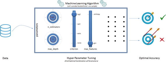
Figure 4-15. Hyperparameter Tuning
GridSearch
For a given model, you can define a set of parameter values that you would like to try. Then using the GridSearchCV function of scikit-learn, models are built for all possible combinations of a preset list of values of hyperparameter provided by you, and the best combination is chosen based on the cross-validation score. There are two disadvantages associated with GridSearchCV.
Computationally expensive: It is then obvious that with more parameter values the GridSearch will be computationally expensive. Consider an example where you have 5 parameters and assume that you would like to try 5 values for each parameters that will result in 5**5 = 3125 combinations; further multiply this with number of cross-validation folds being used, that is, if k-fold is 5 then 3125 * 5 = 15625 model fits.
Not perfect optimal but nearly optimal parameters: Grid Search will look at fixed points that you provide for the numerical parameters, hence there is a great chance of missing the optimal point that lies between the fixed points. For example, assume that you would like to try the fixed points for ‘n_estimators’: [100, 250, 500, 750, 1000] for a decision tree model and there is a chance that the optimal point might lie between the two fixed points; however GridSearch is not designed to search between fixed points.
Let’s try GridSearchCV for a RandomForest classifier on the Pima diabetes dataset to find the optimal parameter values. See Listing 4-21.
Listing 4-21. Grid search for hyperparameter tuning
from sklearn.ensemble import RandomForestClassifierfrom sklearn.grid_search import GridSearchCVseed = 2017# read the data indf = pd.read_csv("Data/Diabetes.csv")X = df.ix[:,:8].values # independent variablesy = df['class'].values # dependent variables#NormalizeX = StandardScaler().fit_transform(X)# evaluate the model by splitting into train and test setsX_train, X_test, y_train, y_test = train_test_split(X, y, test_size=0.3, random_state=seed)kfold = cross_validation.StratifiedKFold(y=y_train, n_folds=5, random_state=seed)num_trees = 100clf_rf = RandomForestClassifier(random_state=seed).fit(X_train, y_train)rf_params = {'n_estimators': [100, 250, 500, 750, 1000],'criterion': ['gini', 'entropy'],'max_features': [None, 'auto', 'sqrt', 'log2'],'max_depth': [1, 3, 5, 7, 9]}# setting verbose = 10 will print the progress for every 10 task completiongrid = GridSearchCV(clf_rf, rf_params, scoring='roc_auc', cv=kfold, verbose=10, n_jobs=-1)grid.fit(X_train, y_train)print 'Best Parameters: ', grid.best_params_results = cross_validation.cross_val_score(grid.best_estimator_, X_train,y_train, cv=kfold)print "Accuracy - Train CV: ", results.mean()print "Accuracy - Train : ", metrics.accuracy_score(grid.best_estimator_.predict(X_train), y_train)print "Accuracy - Test : ", metrics.accuracy_score(grid.best_estimator_.predict(X_test), y_test)#----output----Fitting 5 folds for each of 200 candidates, totalling 1000 fitsBest Parameters: {'max_features': 'log2', 'n_estimators': 500, 'criterion': 'entropy', 'max_depth': 5}Accuracy - Train CV: 0.744790584978Accuracy - Train : 0.862197392924Accuracy - Test : 0.796536796537
RandomSearch
As the name suggests the RandomSearch algorithm tries random combinations of a range of values of given parameters. The numerical parameters can be specified as a range (unlike fixed values in GridSearch). You can control the number of iterations of random searches that you would like to perform. It is known to find a very good combination in a lot less time compared to GridSearch; however you have to carefully choose the range for parameters and the number of random search iteration as it can miss the best parameter combination with lesser iterations or smaller ranges.
Let’s try the RandomSearchCV for same combination that we tried for GridSearch and compare the time / accuracy. See Listing 4-22.
Listing 4-22. Random search for hyperparameter tuning
from sklearn.model_selection import RandomizedSearchCVfrom scipy.stats import randint as sp_randint# specify parameters and distributions to sample fromparam_dist = {'n_estimators':sp_randint(100,1000),'criterion': ['gini', 'entropy'],'max_features': [None, 'auto', 'sqrt', 'log2'],'max_depth': [None, 1, 3, 5, 7, 9]}# run randomized searchn_iter_search = 20random_search = RandomizedSearchCV(clf_rf, param_distributions=param_dist, cv=kfold,n_iter=n_iter_search, verbose=10, n_jobs=-1, random_state=seed)random_search.fit(X_train, y_train)# report(random_search.cv_results_)print 'Best Parameters: ', random_search.best_params_results = cross_validation.cross_val_score(random_search.best_estimator_, X_train,y_train, cv=kfold)print "Accuracy - Train CV: ", results.mean()print "Accuracy - Train : ", metrics.accuracy_score(random_search.best_estimator_.predict(X_train), y_train)print "Accuracy - Test : ", metrics.accuracy_score(random_search.best_estimator_.predict(X_test), y_test)#----output----Fitting 5 folds for each of 20 candidates, totalling 100 fitsBest Parameters: {'max_features': None, 'n_estimators': 694, 'criterion': 'entropy', 'max_depth': 3}Accuracy - Train CV: 0.75424022153Accuracy - Train : 0.780260707635Accuracy - Test : 0.805194805195
Notice that in this case, with RandomSearchCV we were able to achieve comparable accuracy results with 100 fits to that of a GridSearchCV’s 1000 fit.
Figure 4-16 is a sample illustration of how grid search vs. random search results differ (it’s not the actual representation) between two parameters. Assume that the optimal area for max_depth lies between 3 and 5 (blue shade) and for n_estimators it lies between 500 and 700 (amber shade). The ideal optimal value for combined parameters would lie where the individual regions intersect. Both methods will be able to find a nearly optimal parameter and not necessarily the perfect optimal point.
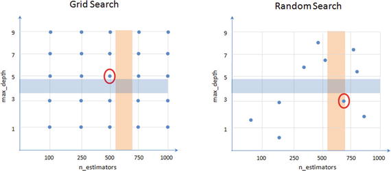
Figure 4-16. Grid Search vs. Random Search
Endnotes
In this step, we have learned various common issues that can hinder the model accuracy such as not choosing the optimal probability cutoff point for class creation, variance, and bias. We also briefly looked at different model tuning techniques practiced such as bagging, boosting, ensemble voting, and grid search/random search for hyperparameter tuning. To be concise we only looked at the most important aspect for each of the topics discussed above to get you started. However there are more options for each of the algorithms for tuning and each of these techniques have been evolving at a fast phase. So I encourage you to keep an eye on their respective officially hosted webpage and github repository. See Table 4-2.
Table 4-2. Additional resources
Name | Web Page | Github Repository |
|---|---|---|
Scikit-learn | ||
Xgboost |
We have reached the end of step 4, which means you’re half way through your machine learning journey. In the next chapter we’ll learn text mining techniques and fundamentals of the recommender system.