- Transforming and drawing 3D objects by applying mathematical functions
- Creating computer animations using transformations to vector graphics
- Identifying linear transformations, which preserve lines and polygons
- Computing the effects of linear transformations on vectors and 3D models
With the techniques from the last two chapters and a little creativity, you can render any 2D or 3D figure you can think of. Whole objects, characters, and worlds can be built from line segments and polygons defined by vectors. But, there’s still one thing standing in between you and your first feature-length, computer-animated film or life-like action video game−you need to be able to draw objects that change over time.
Animation works the same way for computer graphics as it does for film: you render static images and then display dozens of them every second. When we see that many snapshots of a moving object, it looks like the image is continuously changing. In chapters 2 and 3, we looked at a few mathematical operations that take in existing vectors and transform them geometrically to output new ones. By chaining together sequences of small transformations, we can create the illusion of continuous motion.
As a mental model for this, you can keep in mind our examples of rotating 2D vectors. You saw that you could write a Python function, rotate, that took in a 2D vector and rotated it by, say, 45° in the counterclockwise direction. As figure 4.1 shows, you can think of the rotate function as a machine that takes in a vector and outputs an appropriately transformed vector.

Figure 4.1 Picturing a vector function as a machine with an input slot and output slot
If we apply a 3D analogy of this function to every vector of every polygon defining a 3D shape, we can see the whole shape rotate. This 3D shape could be the octahedron from the previous chapter or a more interesting one like a teapot. In figure 4.2, this rotation machine takes a teapot as input and returns a rotated copy as its output.

Figure 4.2 A transformation can be applied to every vector making up a 3D model, thereby transforming the whole model in the same geometric way.
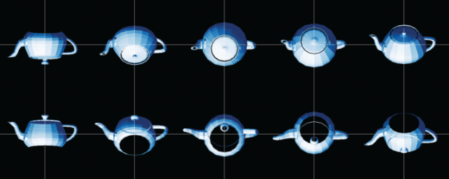
If instead of rotating by 45° once, we rotated by one degree 45 times, we could generate frames of a movie showing a rotating teapot (figure 4.3).
Rotations turn out to be great examples to work with because when we rotate every point on a line segment by the same angle about the origin, we still have a line segment of the same length. As a result, when you rotate all the vectors outlining a 2D or 3D object, you can still recognize the object.

Figure 4.3 Rotating the teapot by 1° at a time, 45 times in a row, beginning with the upper left-hand corner
I’ll introduce you to a broad class of vector transformations called linear transformations that, like rotations, send vectors lying on a straight line to new vectors that also lie on a straight line. Linear transformations have numerous applications in math, physics, and data analysis. It’s helpful to know how to picture them geometrically when you meet them again in these contexts.
To visualize rotations, linear transformations, and other vector transformations in this chapter, we’ll upgrade to more powerful drawing tools. We’ll swap out Matplotlib for OpenGL, which is an industry standard library for high-performance graphics. Most OpenGL programming is done in C or C++, but we’ll use a friendly Python wrapper called PyOpenGL. We’ll also use a video game development library in Python called PyGame. Specifically, we’ll use the features in PyGame that make it easy to render successive images into an animation. The set up for all of these new tools is covered in appendix C, so we can jump right in and focus on the math of transforming vectors. If you want to follow along with the code for this chapter (which I strongly recommend!), then you should skip to appendix C and return here once you get the code working.
4.1 Transforming 3D objects
Our main goal in this chapter is taking a 3D object (like the teapot) and changing it to create a new 3D object that is visually different. In chapter 2, we already saw that we could translate or scale each vector in a 2D dinosaur and the whole dinosaur shape would move or change in size accordingly. We take the same approach here. Every transformation we look at takes a vector as input and returns a vector as output, something like this pseudocode:
def transform(v):
    old_x, old_y, old_z = v
    # ... do some computation here ...
    return (new_x, new_y, new_z)
Let’s start by adapting the familiar examples of translation and scaling from 2D to 3D.
4.1.1 Drawing a transformed object
If you’ve installed the dependencies described in appendix C, you should be able to run the file draw_teapot.py in the source code for chapter 4 (see appendix A for instructions to run a Python script from the command line). If it runs successfully, you should see a PyGame window that shows the image in figure 4.4.

Figure 4.4 The result of running draw_teapot.py
In the next few examples, we modify the vectors defining the teapot and then re-render it so that we can see the geometric effect. As a first example, we can scale all of the vectors by the same factor. The following function, scale2, multiplies an input vector by the scalar 2.0 and returns the result:
from vectors import scale
def scale2(v):
    return scale(2.0, v)
This scale2(v) function has the same form as the transform(v) function given at the top of this section; when passed a 3D vector as input, scale2 returns a new 3D vector as output. To execute this transformation on the teapot, we need to transform each of its vertices. We can do this triangle by triangle. For each triangle that we use to build the teapot, we create a new triangle with the result of applying scale2 to the original vertices:
original_triangles = load_triangles()        ❶
scaled_triangles = [
    [scale2(vertex) for vertex in triangle]  ❷
    for triangle in original_triangles       ❸
]
❶ Loads the triangles using the code from appendix C
❷ Applies scale2 to each vertex in a given triangle to get new vertices
❸ Does this for each triangle in the list of original triangles
Now that we’ve got a new set of triangles, we can draw them by calling draw_model(scaled_triangles). Figure 4.5 shows the teapot after this call, and you can reproduce this by running the file scale_teapot.py in the source code.

Figure 4.5 Applying scale2 to each vertex of each triangle gives us a teapot that is twice as big.
This teapot looks bigger than the original, and in fact, it is twice as big because we multiplied each vector by 2. Let’s apply another transformation to each vector: translation by the vector (−1, 0, 0).
Recall that “translating by a vector” is another way of saying “adding the vector,” so what I’m really talking about is adding (−1, 0, 0) to every vertex of the teapot. This should move the whole teapot one unit in the negative x direction, which is to the left from our perspective. This function accomplishes the translation for a single vertex:
from vectors import add
def translate1left(v):
    return add((−1,0,0), v)
Starting with the original triangles, we now want to scale each of their vertices as before and then apply the translation. Figure 4.6 shows the result. You can reproduce it with the source file scale_translate_teapot.py:
scaled_translated_triangles = [
    [translate1left(scale2(vertex)) for vertex in triangle]
    for triangle in original_triangles
]
draw_model(scaled_translated_triangles)

Figure 4.6 The teapot is bigger and moved to the left as we hoped!
Different scalar multiples change the size of the teapot by different factors, and different translation vectors move the teapot to different positions in space. In the exercises that follow, you’ll have a chance to try different scalar multiples and translations, but for now, let’s focus on combining and applying more transformations.
4.1.2 Composing vector transformations
Applying any number of transformations sequentially defines a new transformation. In the previous section, for instance, we transformed the teapot by scaling it and then translating it. We can package this new transformation as its own Python function:
def scale2_then_translate1left(v):
    return translate1left(scale2(v))
This is an important principle! Because vector transformations take vectors as inputs and return vectors as outputs, we can combine as many of them as we want by composition of functions . If you haven’t heard this term before, it means defining new functions by applying two or more existing ones in a specified order. If we picture the functions scale2 and translate1left as machines that take in 3D models and output new ones (figure 4.7), we can combine them by passing the outputs of the first machine as inputs to the second.

Figure 4.7 Calling scale2 and then translate1left on a teapot to output a transformed version
We can imagine hiding the intermediate step by welding the output slot of the first machine to the input slot of the second machine (figure 4.8).

Figure 4.8 Welding the two function machines together to get a new one, which performs both transformations in one step
We can think of the result as a new machine that does the work of both the original functions in one step. This “welding” of functions can be done in code as well. We can write a general-purpose compose function that takes two Python functions (for vector transformations, for instance) and returns a new function, which is their composition:
def compose(f1,f2):
    def new_function(input):
        return f1(f2(input))
    return new_function
Instead of defining scale2_then_translate1left as its own function, we could write
scale2_then_translate1left = compose(translate1left, scale2)
You might have heard of the idea that Python treats functions as “first-class objects.” What is usually meant by this slogan is that Python functions can be assigned to variables, passed as inputs to other functions, or created on-the-fly and returned as output values. These are functional programming techniques, meaning that they help us build complex programs by combining existing functions to make new ones.
There is some debate about whether functional programming is kosher in Python (or as a Python fan would say, whether or not functional programming is “Pythonic”). I won’t opine about coding style, but I use functional programming because functions, namely vector transformations, are our central objects of study. With the compose function covered, I’ll show you a few more functional “recipes” that justify this digression. Each of these is added in a new helper file called transforms.py in the source code for this book.
Something we’ll be doing repeatedly is taking a vector transformation and applying it to every vertex in every triangle defining a 3D model. We can write a reusable function for this rather than writing a new list comprehension each time. The following polygon_map function takes a vector transformation and a list of polygons (usually triangles) and applies the transformation to each vertex of each polygon, yielding a new list of new polygons:
def polygon_map(transformation, polygons):
    return [
        [transformation(vertex) for vertex in triangle]
        for triangle in polygons
    ]
With this helper function, we can apply scale2 to the original teapot in one line:
draw_model(polygon_map(scale2, load_triangles()))
The compose and polygon_map functions both take vector transformations as arguments, but it’s also useful to have functions that return vector transformations. For instance, it might have bothered you that we named a function scale2 and hard-coded the number two into its definition. A replacement for this could be a scale_by function that returns a scaling transformation for a specified scalar:
def scale_by(scalar):
    def new_function(v):
        return scale(scalar, v)
    return new_function
With this function, we can write scale_by(2) and the return value would be a new function that behaves identically to scale2. While we’re picturing functions as machines with input and output slots, you can picture scale_by as a machine that takes numbers in its input slot and outputs new function machines from its output slot as shown in figure 4.9.

Figure 4.9 A function machine that takes numbers as inputs and produces new function machines as outputs
As an exercise, you can write a similar translate_by function that takes a translation vector as input and returns a translation function as output. In the terminology of functional programming, this process is called currying . Currying takes a function that accepts multiple inputs and refactors it to a function that returns another function.
The result is a programmatic machine that behaves identically but is invoked differently; for instance, scale_by(s)(v) gives the same result as scale(s,v) for any inputs s and v. The advantage is that scale(...) and add(...) accept different kinds of arguments, so the resulting functions, scale_by(s) and translate _by(w), are interchangeable. Next, we’ll think similarly about rotations: for any given angle, we can produce a vector transformation that rotates our model by that angle.
4.1.3 Rotating an object about an axis
You already saw how to do rotations in 2D in chapter 2: you convert the Cartesian coordinates to polar coordinates, increase or decrease the angle by the rotation factor, and then convert back. Even though this is a 2D trick, it is helpful in 3D because all 3D
vector rotations are, in a sense, isolated in planes. Picture, for instance, a single point in 3D being rotated about the z -axis. Its x − and y-coordinates change, but its z-coordinate remains the same. If a given point is rotated around the z -axis, it stays in a circle with a constant z-coordinate, regardless of the rotation angle (figure 4.10).

Figure 4.10 Rotating a point around the z-axis
What this means is that we can rotate a 3D point around the z -axis by holding the z-coordinate constant and applying our 2D rotation function only to the x − and y-coordinates. We’ll work through the code here, and you can also find it in rotate_teapot.py in the source code. First, we write a 2D rotation function adapted from the strategy we used in chapter 2:
def rotate2d(angle, vector):
    l,a = to_polar(vector)
    return to_cartesian((l, a+angle))
This function takes an angle and a 2D vector and returns a rotated 2D vector. Now, let’s create a function, rotate_z, that applies this function only to the x and y components of a 3D vector:
def rotate_z(angle, vector):
    x,y,z = vector
    new_x, new_y = rotate2d(angle, (x,y))
    return new_x, new_y, z
Continuing to think in the functional programming paradigm, we can curry this function. Given any angle, the curried version produces a vector transformation that does the corresponding rotation:
def rotate_z_by(angle):
    def new_function(v):
        return rotate_z(angle,v)
    return new_function
Let’s see it in action. The following line yields the teapot in figure 4.11, which is rotated by π/4 or 45°:
draw_model(polygon_map(rotate_z_by(pi/4.), load_triangles()))

Figure 4.11 The teapot is rotated 45° counterclockwise about the z-axis.
We can write a similar function to rotate the teapot about the x-axis, meaning the rotation affects only the y and z components of the vector:
def rotate_x(angle, vector):
    x,y,z = vector
    new_y, new_z = rotate2d(angle, (y,z))
    return x, new_y, new_z
def rotate_x_by(angle):
    def new_function(v):
        return rotate_x(angle,v)
    return new_function
In the function rotate_x_by, a rotation about the x-axis is achieved by fixing the x coordinate and executing a 2D rotation in the y,z plane. The following code draws a 90° or π/2 radian rotation (counterclockwise) about the x-axis, resulting in the upright teapot shown in figure 4.12:
draw_model(polygon_map(rotate_x_by(pi/2.), load_triangles()))

Figure 4.12 The teapot rotated by π/2 about the x-axis.
You can reproduce figure 4.12 with the source file rotate_teapot_x.py. The shading is consistent among these rotated teapots; their brightest polygons are toward the top-right of the figures, which is expected because the light source remains at (1, 2, 3). This is a good sign that we are successfully moving the teapot and not just changing our OpenGL perspective as before.
It turns out that it’s possible to get any rotation we want by composing rotations in the x and z directions. In the exercises at the end of the section, you can try your hand at some more rotations, but for now, we’ll move on to other kinds of vector transformations.
4.1.4 Inventing your own geometric transformations
So far, I’ve focused on the vector transformations we already saw in some way in the preceding chapters. Now, let’s throw caution to the wind and see what other interesting transformations we can come up with. Remember, the only requirement for a 3D vector transformation is that it accepts a single 3D vector as input and returns a new 3D vector as its output. Let’s look at a few transformations that don’t quite fall in any of the categories we’ve seen so far.
For our teapot, let’s modify one coordinate at a time. This function stretches vectors by a (hard-coded) factor of four, but only in the x direction:
def stretch_x(vector):
    x,y,z = vector
    return (4.*x, y, z)
The result is a long, skinny teapot along the x-axis or in the handle-to-spout direction (figure 4.13). This is fully implemented in stretch_teapot.py.

Figure 4.13 A teapot stretched along the x-axis.
A similar stretch_y function elongates the teapot from top-to-bottom. You can implement stretch_y and apply it to a teapot yourself, and you should get the image in figure 4.14. Otherwise, you can look at the implementation in stretch_teapot_y.py in the source code.
We can get even more creative, stretching the teapot by cubing the y-coordinate rather than just multiplying it by a number. This transformation gives the teapot a disproportionately elongated lid as implemented in cube_teapot.py and shown in figure 4.15:
def cube_stretch_z(vector):
    x,y,z = vector
    return (x, y*y*y, z)

Figure 4.14 Stretching the teapot in the y direction instead

Figure 4.15 Cubing the vertical dimension of the teapot
If we selectively add two of the three coordinates in the formula for the transformation, for instance the x and y coordinates, we can cause the teapot to slant. This is implemented in slant_teapot.py and shown in figure 4.16:

Figure 4.16 Adding the y-coordinate to the existing x-coordinate causes the teapot to slant in the x direction.
def slant_xy(vector):
    x,y,z = vector
    return (x+y, y, z)
The point is not that any one of these transformations is important or useful, but that any mathematical transformation of the vectors constituting a 3D model have some geometric consequence on the appearance of the model. It is possible to go too crazy with the transformation, at which point the model can become too distorted to recognize or even to draw successfully. Indeed, some transfor-mations are better-behaved in general, and we’ll classify them in the next section.
4.1.5 Exercises
def translate_by(translation):
    def new_function(v):
        return add(translation,v)
    return new_function
|
draw_model(polygon_map(translate_by((0,0,−20)), load_triangles()))
The teapot translated 20 units down the z-axis. It appears smaller because it is further from the viewpoint. |


draw_model(polygon_map(compose(scale2, translate1left), load_triangles()))
Scaling and then translating the teapot (left) vs. translating and then scaling (right) |

def prepend(string):
    def new_function(input):
        return string + input
    return new_function

f = compose(prepend("P"), prepend("y"), prepend("t"))
|
def curry2(f):
    def g(x):
        def new_function(y):
            return f(x,y)
        return new_function
    return g
>>> scale_by = curry2(scale) >>> scale_by(2)((1,2,3)) (2, 4, 6) |
def stretch_x(scalar,vector):
    x,y,z = vector
    return (scalar*x, y, z)

def stretch_x_by(scalar):
    def new_function(vector):
        return stretch_x(scalar,vector)
    return new_function
|
4.2 Linear transformations
The well-behaved vector transformations we’re going to focus on are called linear transformations. Along with vectors, linear transformations are the other main objects of study in linear algebra. Linear transformations are special transformations where vector arithmetic looks the same before and after the transformation. Let’s draw some diagrams to show exactly what that means.
4.2.1 Preserving vector arithmetic
The two most important arithmetic operations on vectors are addition and scalar multiplication. Let’s return to our 2D pictures of these operations and see how they look before and after a transformation is applied.
We can picture the sum of two vectors as the new vector we arrive at when we place them tip-to-tail, or as the vector to the tip of the parallelogram they define. For instance, figure 4.17 represents the vector sum u + v = w.

Figure 4.17 Geometric demonstration of the vector sum z + v = w
The question we want to ask is, if we apply the same vector transformation to all three of the vectors in this diagram, will it still look like a vector sum? Let’s try a vector transformation, which is a counterclockwise rotation about the origin, and call this transformation R. Figure 4.18 shows u, v, and w rotated by the same angle by the transformation R.
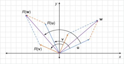
Figure 4.18 After rotating u, v, and w by the same rotation R, the sum still holds.
The rotated diagram is exactly the diagram representing the vector sum R(u) + R(v) = R(w). You can draw the picture for any three vectors u, v, and w, and as long as u + v = w and if you apply the same rotation transformation R to each of the vectors, you find that R(u) + R(v) = R(w) as well. To describe this property, we say that rotations preserve vector sums.
Similarly, rotations preserve scalar multiples. If v is a vector and sv is a multiple of v by a scalar s, then sv points in the same direction but is scaled by a factor of s. If we rotate v and sv by the same rotation R, we’ll see that R(s v) is a scalar multiple of R(v) by the same factor s(figure 4.19).

Figure 4.19 Scalar multiplication is preserved by rotation.
Again, this is only a visual example and not a proof, but you’ll find that for any vector v, scalar s, and rotation R, the same picture holds. Rotations or any other vector transformations that preserve vector sums and scalar multiples are called linear transformations.
Make sure you pause to digest this definition; linear transformations are so important that the whole subject of linear algebra is named after them. To help you recognize linear transformations when you see them, we’ll look at a few more examples.
4.2.2 Picturing linear transformations
First, let’s look at a counterexample: a vector transformation that’s not linear. Such an example is a transformation S(v) that takes a vector v = (x, y) and outputs a vector with both coordinates squared: S(v) = (x2, y2). As an example, let’s look at the sum of u = (2, 3) and v = (1, −1). The sum is (2, 3) + (1, −1) = (3, 2). This is shown with vector addition in figure 4.20.

Figure 4.20 Picturing the vector sum of z = (2, 3) and v = (1, −1), z + v = (3, 2)
Now let’s apply S to each of these: S(u) = (4, 9), S(v) = (1, 1), and S(u + v) = (9, 4). Figure 4.21 clearly shows that S(u) + S(v) does not agree with S(u + v).

Figure 4.21 S does not respect sums! S(u) + S(v) is far from S(u + v).
As an exercise, you can try to find a counterexample demonstrating that S does not preserve scalar multiples either. For now, let’s examine another transformation. Let D(v) be the vector transformation that scales the input vector by a factor of 2. In other words, D(v) = 2v. This does preserve vector sums: if u + v = w, then 2u + 2v = 2w as well. Figure 4.22 provides a visual example.

Figure 4.22 Doubling the lengths of vectors preserves their sums: if z + v = w, then D(u) + D(v) = D(w)
Likewise, D(v) preserves scalar multiplication. This is a bit harder to draw, but you can see it algebraically. For any scalar s, D(sv) = 2(sv) = s(2v) = sD(v).
How about translation? Suppose B(v) translates any input vector v by (7, 0). Surprisingly, this is not a linear transformation. Figure 4.23 provides a visual counterexample where u + v = w, but B(v) + B(w) is not the same as B(v + w).
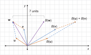
Figure 4.23 The translation transformation B does not preserve a vector sum because B(u) + B(v) is not equal to B(u + v).
It turns out that for a transformation to be linear, it must not move the origin (see why as an exercise later). Translation by any non-zero vector transforms the origin, which ends up at a different point, so it cannot be linear.
Other examples of linear transformations include reflection, projection, shearing, and any 3D analogy of the preceding linear transformations. These are defined in the exercises section and you should convince yourself with several examples that each of these transformations preserves vector addition and scalar multiplication. With practice, you can recognize which transformations are linear and which are not. Next, we’ll look at why the special properties of linear transformations are useful.
4.2.3 Why linear transformations?
Because linear transformations preserve vector sums and scalar multiples, they also preserve a broader class of vector arithmetic operations. The most general operation is called a linear combination . A linear combination of a collection of vectors is a sum of scalar multiples of them. For instance, one linear combination of two vectors u and v would be 3u − 2v. Given three vectors u, v, and w , the expression 0.5u − v + 6 w is a linear combination of u , v , and w. Because linear transformations preserve vector sums and scalar multiples, these preserve linear combinations as well.
We can restate this fact algebraically. If you have a collection of n vectors, v1, v2, ..., v n, as well as any choice of n scalars, s1, s2, s3, ..., sn, a linear transformation T preserves the linear combination:
T(s1 v1 + s2 v2 + s3 v3 + ... + snvn) = s1 T(v1) + s2 T(v2) + s3 T(v3) + ... + snT(vn)
One easy-to-picture linear combination we’ve seen before is ½ u + ½ v for vectors u and v, which is equivalent to ½ (u + v). Figure 4.24 shows that this linear combination of two vectors gives us the midpoint of the line segment connecting them.

Figure 4.24 The midpoint between the tips of two vectors z and v can be found as the linear combination ½ z + ½ v = ½ (u + v).
This means linear transformations send midpoints to other midpoints: for example, T(½ u + ½ v) = ½ T(u) + ½ T(v), which is the midpoint of the segment connecting T(u) and T(v) as figure 4.25 shows.

Figure 4.25 Because the midpoint between two vectors is a linear combination of the vectors, the linear transformation T sets the midpoint between z and v to the midpoint between T(u) and T(v).
It’s less obvious, but a linear combination like 0.25u + 0.75v also lies on the line segment between u and v (figure 4.26). Specifically, this is the point 75% of the way from u to v. Likewise, 0.6u + 0.4v is 40% of the way from u to v, and so on.

Figure 4.26 The point 0.25u + 0.75v lies on the line segment connecting z and v, 75% of the way from z to v. You can see this concretely with u = (−2, 2) and v = (6, 6).
In fact, every point on the line segment between two vectors is a “weighted average” like this, having the form su + (1 − s)v for some number s between 0 and 1. To convince you, figure 4.27 shows the vectors su + (1 − s)v for u = (−1, 1) and v = (3, 4) for 10 values of s between 0 and 1 and then for 100 values of s between 0 and 1.


Figure 4.27 Plotting various weighted averages of (−1, 1) and (3, 4) with 10 values of s between 0 and 1 (left) and 100 values of s between 0 and 1 (right)
The key idea here is that every point on a line segment connecting two vectors u and v is a weighted average and, therefore, a linear combination of points u and v. With this in mind, we can think about what a linear transformation does to a whole line segment.
Any point on the line segment connecting u and v is a weighted average of u and v, so it has the form s · u + (1 − s) · v for some value s. A linear transformation, T, transforms u and v to some new vectors T(u) and T(v). The point on the line segment is transformed to some new point T(s · u + (1 − s) · v) or s · T(u) + (1 − s) · T(v). This is, in turn, a weighted average of T(u) and T(v), so it is a point that lies on the segment connecting T(u) and T(v) as shown in figure 4.28.

Figure 4.28 A linear transformation T transforms a weighted average of z and v to a weighted average of T(u) and T(v). The original weighted average lies on the segment connecting z and v, and the transformed one lies on the segment connecting T(u) and T(v).
Because of this, a linear transformation T takes every point on the line segment connecting u and v to a point on the line segment connecting T(u) and T(v). This is a key property of linear transformations: they send every existing line segment to a new line segment. Because our 3D models are made up of polygons and polygons are outlined by line segments, linear transformations can be expected to preserve the structure of our 3D models to some extent (figure 4.29).
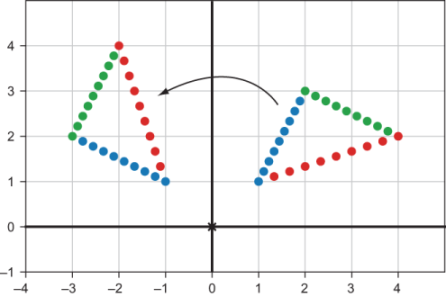
Figure 4.29 Applying a linear transformation (rotation by 60°) to points making up a triangle. The result is a rotated triangle (on the left).
By contrast, if we use the non-linear transformation S(v) sending v = (x, y) to (x2, y2), we can see that line segments are distorted. This means that a triangle defined by vectors u, v, and w is not really sent to another triangle defined by S(u), S(v), and S(w) as shown in figure 4.30.

Figure 4.30 Applying the non-linear transformation S does not preserve the straightness of edges of the triangle.
In summary, linear transformations respect the algebraic properties of vectors, preserving sums, scalar multiples, and linear combinations. They also respect the geometric properties of collections of vectors, sending line segments and polygons defined by vectors to new ones defined by the transformed vectors. Next, we’ll see that linear transformations are not only special from a geometric perspective; they’re also easy to compute.
4.2.4 Computing linear transformations
In chapters 2 and 3, you saw how to break 2D and 3D vectors into components. For instance, the vector (4, 3, 5) can be decomposed as a sum (4, 0, 0) + (0, 3, 0) + (0, 0, 5). This makes it easy to picture how far the vector extends in each of the three dimensions of the space that we’re in. We can decompose this even further into a linear combination (figure 4.31):
(4, 3, 5) = 4 · (1, 0, 0) + 3 · (0, 1, 0) + 5 · (0, 0, 1)

Figure 4.31 The 3D vector (4, 3, 5) as a linear combination of (1, 0, 0), (0, 1, 0), and (0, 0, 1)
This might seem like a boring fact, but it’s one of the profound insights from linear algebra: any 3D vector can be decomposed into a linear combination of three vectors (1, 0, 0), (0, 1, 0), and (0, 0, 1). The scalars appearing in this decomposition for a vector v are exactly the coordinates of v.
The three vectors (1, 0, 0), (0, 1, 0), and (0, 0, 1) are called the standard basis for three-dimensional space. These are denoted e1, e2, and e3, so we could write the previous linear combination as (3, 4, 5) = 3 e1 + 4 e2 + 5 e3. When we’re working in 2D space, we call e1 = (1, 0) and e2 = (0, 1); so, for example, (7, −4) = 7 e1 − 4 e2(figure 4.32). (When we say e1, we could mean (1, 0) or (1, 0, 0), but usually it’s clear which one we mean once we’ve established whether we’re working in two or three dimensions.)

Figure 4.32 The 2D vector (7, −4) as a linear combination of the standard basis vectors e1 and e2
We’ve only written the same vectors in a slightly different way, but it turns out this change in perspective makes it easy to compute linear transformations. Because linear transformations respect linear combinations, all we need to know to compute a linear transformation is how it affects standard basis vectors.
Let’s look at a visual example (figure 4.33). Say we know nothing about a 2D vector transformation T except that it is linear and we know what T(e1) and T(e2) are.

Figure 4.33 When a linear transformation acts on the two standard basis vectors in 2D, we get two new vectors as a result.
For any other vector v, we automatically know where T(v) ends up. Say v = (3, 2), then we can assert:
T(v) = T(3e1 + 2e2) = 3T(e1) + 2T(e2)
Because we already know where T(e1) and T(e2) are, we can locate T(v) as shown in figure 4.34.

Figure 4.34 We can compute T(v) for any vector v as a linear combination of T(e1) and T(e2).
To make this more concrete, let’s do a complete example in 3D. Say a is a linear transformation, and all we know about a is that a(e1) = (1, 1, 1), a(e2) = (1, 0, −1), and a(e3) = (0, 1, 1). If v = (−1, 2, 2), what is a(v)? Well, first we can expand v as a linear combination of the three standard basis vectors. Because v = (−1, 2, 2) = −e1 + 2e2 + 2e3, we can make the substitution:
Next, we can use the fact that a is linear and preserves linear combinations:
Finally, we can substitute in the known values of a(e1), a(e2), and a(e3), and simplify:
= − (1, 1, 1) + 2 · (1, 0, −1) + 2 · (0, 1, 1)
As proof we really know how a works, we can apply it to the teapot:
Ae1 = (1,1,1)                                        ❶
Ae2 = (1,0,−1)
Ae3 = (0,1,1)

def apply_A(v):                                      ❷
    return add(                                      ❸
        scale(v[0], Ae1),
        scale(v[1], Ae2),
        scale(v[2], Ae3)
    )

draw_model(polygon_map(apply_A, load_triangles()))   ❹
❶ The known results of applying A to the standard basis vectors
❷ Builds a function apply_A(v) that returns the result of A on the input vector v
❸ The result should be a linear combination of these vectors, where the scalars are taken to be the coordinates of the target vector v.
❹ Uses polygon_map to apply A to every vector of every triangle in the teapot
Figure 4.35 shows the result of this transformation.

Figure 4.35 In this rotated, skewed configuration, we see that the teapot does not have a bottom!
The takeaway here is that a 2D linear transformation T is defined completely by the values of T(e1) and T(e2); that’s two vectors or four numbers in total. Likewise, a 3D linear transformation T is defined completely by the values of T(e1), T(e2), and T(e3), which are three vectors or nine numbers in total. In any number of dimensions, the behavior of a linear transformation is specified by a list of vectors or an array-of-arrays of numbers. Such an array-of-arrays is called a matrix, and we’ll see how to use matrices in the next chapter.
4.2.5 Exercises
|
The midpoint of the segment connecting (5, 3) and (−2, 1) is (3/2, 2). |

|
The grid of points is initially uniformly spaced, but after applying the transformation S, the spacing varies between points, even on the same lines. |


|
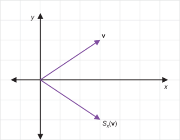
A vector v = (3, 2) and its reflection over the x-axis (3, −2) |
|
For z + v = w as shown, reflection over the x-axis preserves the sum; that is, Sx(u) + Sx(v) = Sx(w).
Reflection across the x-axis preserves this scalar multiple. |


|
A quarter-turn counterclockwise in the y,z plane sends e2 to e3 and e3 to − e2. |

from vectors import *
def linear_combination(scalars,*vectors):
    scaled = [scale(s,v) for s,v in zip(scalars,vectors)]
    return add(*scaled)
>>> linear_combination([1,2,3], (1,0,0), (0,1,0), (0,0,1)) (1, 2, 3) |
def transform_standard_basis(transform):
    return transform((1,0,0)), transform((0,1,0)), transform((0,0,1))
>>> from math import *
>>> transform_standard_basis(rotate_x_by(pi/2))
((1, 0.0, 0.0), (0, 6.123233995736766e−17, 1.0), (0, −1.0,
    1.2246467991473532e−16))
|
Linear transformations are both well-behaved and easy-to-compute because these can be specified with so little data. We explore this more in the next chapter when we compute linear transformations with matrix notation.
Summary
-
Vector transformations are functions that take vectors as inputs and return vectors as outputs. Vector transformations can operate on 2D or 3D vectors.
-
To effect a geometric transformation of the model, apply a vector transformation to every vertex of every polygon of a 3D model.
-
You can combine existing vector transformations by composition of functions to create new transformations, which are equivalent to applying the existing vector transformations sequentially.
-
Functional programming is a programming paradigm that emphasizes composing and, otherwise, manipulating functions.
-
The functional operation of currying turns a function that takes multiple arguments into a function that takes one argument and returns a new function. Currying lets you turn existing Python functions (like
scaleandadd) into vector transformations. -
Linear transformations are vector transformations that preserve vector sums and scalar multiples. In particular, points lying on a line segment still lie on a line segment after a linear transformation is applied.
-
A linear combination is the most general combination of scalar multiplication and vector addition. Every 3D vector is a linear combination of the 3D standard basis vectors, which are denoted e1 = (1, 0, 0), e2 = (0, 1, 0), and e3 = (0, 0, 1). Likewise, every 2D vector is a linear combination of the 2D standard basis vectors, which are e1 = (1, 0) and e2 = (0, 1).
-
Once you know how a given linear transformation acts on the standard basis vectors, you can determine how it acts on any vector by writing the vector as a linear combination of the standard basis and using the fact that linear combinations are preserved.
- In 3D, three vectors or nine total numbers specify a linear transformation.
- In 2D, two vectors or four total numbers do the same.
This last point is critical: linear transformations are both well-behaved and easy-to-compute with because they can be specified with so little data.