This chapter covers

• Implementing a Python abstract base class for general vectors
• Defining vector spaces and listing their useful properties
• Interpreting functions, matrices, images, and sound waves as vectors
• Finding useful subspaces of vector spaces containing data of interest

Even if you’re not interested in animating teapots, the machinery of vectors, linear transformations, and matrices can still be useful. In fact, these concepts are so useful there’s an entire branch of math devoted to them: linear algebra. Linear algebra generalizes everything we know about 2D and 3D geometry to study data in any number of dimensions.

As a programmer, you’re probably skilled at generalizing ideas. When writing complex software, it’s common to find yourself writing similar code over and over. At some point, you catch yourself doing this, and you consolidate the code into one class or function capable of handling all of the cases you see. This saves you typing and often improves code organization and maintainability. Mathematicians follow the same process: after encountering similar patterns over and over, they can better state exactly what they see and refine their definitions.

In this chapter, we use this kind of logic to define vector spaces. Vector spaces are collections of objects we can treat like vectors. These can be arrows in the plane, tuples of numbers, or objects completely different from the ones we’ve seen so far. For instance, you can treat images as vectors and take a linear combination of them (figure 6.1).

Figure 6.1 A linear combination of two pictures produces a new picture.

The key operations in a vector space are vector addition and scalar multiplication. With these, you can make linear combinations (including negation, subtraction, weighted averages, and so on), and you can reason about which transformations are linear. It turns out these operations help us make sense of the word dimension. For instance, we’ll see that the images used in figure 6.1 are 270,000-dimensional objects! We’ll cover higher-dimensional and even infinite-dimensional spaces soon enough, but let’s start by reviewing the 2D and 3D spaces we already know.

6.1 Generalizing our definition of vectors

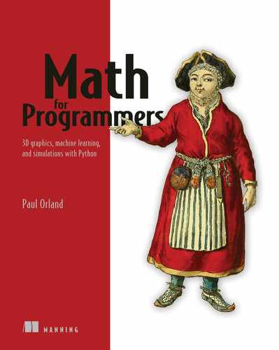
Python supports object-oriented programming (OOP), which is a great framework for generalization. Specifically, Python classes support inheritance : you can create new classes of objects that inherit properties and behaviors of an existing parent class. In our case, we want to realize the 2D and 3D vectors we’ve already seen as instances of a more general class of objects simply called vectors. Then any other objects that inherit behaviors from the parent class can rightly be called vectors as well (figure 6.2).

Figure 6.2 Treating 2D vectors, 3D vectors, and other objects as special cases of vectors using inheritance

If you haven’t done object-oriented programming or you haven’t seen it done in Python, don’t worry. I stick to simple use cases in this chapter and will help you pick it up as we go. In case you want to learn more about classes and inheritance in Python before getting started, I’ve covered them in appendix B.

6.1.1 Creating a class for 2D coordinate vectors

In code, our 2D and 3D vectors have been coordinate vectors, meaning that they were defined as tuples of numbers, which are their coordinates. (We also saw that vector arithmetic can be defined geometrically in terms of arrows, but we can’t translate that approach directly into Python code.) For 2D coordinate vectors, the data is the ordered pair of the x − and y-coordinates. A tuple is a great way to store this data, but we can equivalently use a class. We’ll call the class representing 2D coordinate vectors Vec2 :

class Vec2():
    def __init__(self,x,y):
        self.x = x
        self.y = y

We can initialize a vector like v = Vec2(1.6,3.8) and retrieve its coordinates as v.x and v.y. Next, we can give this class the methods required to do 2D vector arithmetic, specifically addition and scalar multiplication. The addition function, add, takes a second vector as an argument and returns a new Vec2 object whose coordinates are the sum of the x − and y-coordinates, respectively:

class Vec2():
    ...                 ❶
    def add(self, v2):
        return Vec2(self.x + v2.x, self.y + v2.y)

❶ When adding to an existing class, I sometimes use ... as a placeholder for existing code.

Doing vector addition with Vec2 could look like this:

v = Vec2(3,4)          ❶
w = v.add(Vec2(−2,6))  ❷
print(w.x)             ❸

❶ Creates a new Vec2 called v with an x-coordinate 3 and y-coordinate 4

❷ Adds a second Vec2 to v to produce a new Vec2 instance called w. This operation returns (3,4) + (−2,6) = (1,10).

❸ Prints the x-coordinate of w. The result is 1.

Like our original implementation of vector addition, we do not perform the addition “in-place.” That is, the two input vectors are not modified; a new Vec2 object is created to store the sum. We can implement scalar multiplication in a similar way, taking a scalar as input and returning a new, scaled vector as output:

class Vec2():
    ...
    def scale(self, scalar):
        return Vec2(scalar * self.x, scalar * self.y)

Vec(1,1).scale(50) returns a new vector with the x -and y-coordinates both equal to 50. There’s one more critical detail we need to take care of: currently the output of a comparison like Vec2(3,4) == Vec2(3,4) is False. This is problematic because these instances represent the same vector. By default, Python compares instances by their references (asking whether they are located in the same place in memory) rather than by their values. We can fix this by overriding the equality method, which causes Python to treat the == operator differently for objects of the Vec2 class. (If you haven’t seen this before, appendix B explains it in more depth.)

class Vec2():
    ...
    def __eq__(self,other):
        return self.x == other.x and self.y == other.y

We want two 2D coordinate vectors to be equal if their x − and y-coordinates agree, and this new definition of equality captures that. With this implemented, you’ll find that Vec2(3,4) == Vec2(3,4).

Our Vec2 class now has the fundamental vector operations of addition and scalar multiplication, as well as an equality test that makes sense. We can now turn our attention to some syntactic sugar.

6.1.2 Improving the Vec2 class

As we changed the behavior of the == operator, we can also customize the Python operators + and * to mean vector addition and scalar multiplication, respectively. This is called operator overloading, and it is covered in appendix B:

class Vec2():
    ...
    def __add__(self, v2):
        return self.add(v2)
    def __mul__(self, scalar):     ❶
        return self.scale(scalar)
    def __rmul__(self,scalar): 
        return self.scale(scalar)

❶ The __mul__ and __rmul__ methods define both orders of multiplication, so we can multiply vectors by scalars on the left or the right. Mathematically, we consider both orders to mean the same thing.

We can now write a linear combination concisely. For instance, 3.0 * Vec2(1,0) + 4.0 * Vec2(0,1) gives us a new Vec2 object with x-coordinate 3.0 and y-coordinate 4.0. It’s hard to read this in an interactive session though, because Python doesn’t print Vec2 nicely:

>>> 3.0 * Vec2(1,0) + 4.0 * Vec2(0,1)
<__main__.Vec2 at 0x1cef56d6390>

Python gives us the memory address of the resulting Vec2 instance, but we already observed that’s not what’s important to us. Fortunately, we can change the string representation of Vec2 objects by overriding the __repr__ method:

class Vec2():
    ...
    def __repr__(self):
        return "Vec2({},{})".format(self.x,self.y)

This string representation shows the coordinates that are the most important data for a Vec2 object. The results of Vec2 arithmetic are much clearer now:

>>> 3.0 * Vec2(1,0) + 4.0 * Vec2(0,1)
Vec2(3.0,4.0)

We’re doing the same math here as we did with our original tuple vectors but, in my opinion, this is a lot nicer. Building a class required some boilerplate, like the custom equality we wanted, but it also enabled operator overloading for vector arithmetic. The custom string representation also makes it clear that we’re not just working with any tuples, but rather 2D vectors that we intend to use in a certain way. Now, we can implement 3D vectors represented by their own special class.

6.1.3 Repeating the process with 3D vectors

I’ll call the 3D vector class Vec3, and it looks a lot like the 2D Vec2 class except that its defining data will be three coordinates instead of two. In each method that explicitly references the coordinates, we need to make sure to properly use the x, y, and z values for Vec3.

class Vec3():
    def __init__(self,x,y,z): #1
        self.x = x
        self.y = y
        self.z = z
    def add(self, other):
        return Vec3(self.x + other.x, self.y + other.y, self.z + other.z)
    def scale(self, scalar):
        return Vec3(scalar * self.x, scalar * self.y, scalar * self.z)
    def __eq__(self,other):
        return (self.x == other.x 
                and self.y == other.y 
                and self.z == other.z)
    def __add__(self, other):
        return self.add(other)
    def __mul__(self, scalar):
        return self.scale(scalar)
    def __rmul__(self,scalar):
        return self.scale(scalar)
    def __repr__(self):
        return "Vec3({},{},{})".format(self.x,self.y, self.z)

We can now write 3D vector math in Python using the built-in arithmetic operators:

>>> 2.0 * (Vec3(1,0,0) + Vec3(0,1,0))
Vec3(2.0,2.0,0.0)

This Vec3 class, much like the Vec2 class, puts us in a good place to think about generalization. There are a few different directions we can go, and like many software design choices, the decision is subjective. We could, for example, focus on simplifying the arithmetic. Instead of implementing add differently for Vec2 and Vec3, they can both use the add function we built in chapter 3, which already handles coordinate vectors of any size. We could also store coordinates internally as a tuple or list, letting the constructor accept any number of coordinates and create a 2D, 3D, or other coordinate vector. I’ll leave these possibilities as exercises for you, however, and take us in a different direction.

The generalization I want to focus on is based on how we use the vectors, not on how they work. This gets us to a mental model that both organizes the code well and aligns with the mathematical definition of a vector. For instance, we can write a generic average function that can be used on any kind of vector:

def average(v1,v2):
    return 0.5 * v1 + 0.5 * v2

We can insert either 3D vectors or 2D vectors; for instance, average(Vec2(9.0, 1.0), Vec2(8.0,6.0)) and average(Vec3(1,2,3), Vec3(4,5,6)) both give us correct and meaningful results. As a spoiler, we will soon be able to average pictures together as well. Once we’ve implemented a suitable class for images, we’ll be able to write average(img1, img2) and get a new image back.

This is where we see the beauty and the economy that comes with generalization. We can write a single, generic function like average and use it for a wide variety of types of inputs. The only constraint on the input is that it needs to support multiplication by scalars and addition with one another. The implementation of arithmetic varies between Vec2 objects, Vec3 objects, images, or other kinds of data, but there’s always an important overlap in what arithmetic we can do with them. When we separate the what from the how, we open the door for code reuse and far-reaching mathematical statements.

How can we best describe what we can do with vectors separately from the details of how we carry them out? We can capture this in Python using an abstract base class.

6.1.4 Building a vector base class

The basic things we can do with Vec2 or Vec3 include constructing a new instance, adding with other vectors, multiplying by a scalar, testing equality with another vector, and representing an instance as a string. Of these, only addition and scalar multiplication are distinctive vector operations. Any new Python class automatically includes the rest. This prompts a definition of a Vector base class:

from abc import ABCMeta, abstractmethod

class Vector(metaclass=ABCMeta):
    @abstractmethod
    def scale(self,scalar):
        pass
    @abstractmethod
    def add(self,other):
        pass

The abc module contains helper classes, functions, and method decorators that help define an abstract base class, a class that is not intended to be instantiated. Instead, it’s designed to be used as a template for classes that inherit from it. The @abstractmethod decorator means that a method is not implemented in the base class and needs to be implemented for any child class. For instance, if you try to instantiate a vector with code like v = Vector(), you get the following TypeError :

TypeError: Can't instantiate abstract class Vector with abstract methods add, scale

This makes sense; there is no such thing as a vector that is “just a vector.” It needs to have some concrete manifestation such as a list of coordinates, an arrow in the plane, or something else. But this is still a useful base class because it forces any child class to include requisite methods. It is also useful to have this base class because we can equip it with all the methods that depend only on addition and scalar multiplication, like our operator overloads:

class Vector(metaclass=ABCMeta):
    ...
    def __mul__(self, scalar):
        return self.scale(scalar)
    def __rmul__(self, scalar):
        return self.scale(scalar)
    def __add__(self,other):
        return self.add(other)

In contrast to the abstract methods scale and add, these implementations are automatically available to any child class. We can simplify Vec2 and Vec3 to inherit from Vector. Here’s a new implementation for Vec2 :

class Vec2(Vector):
    def __init__(self,x,y):
        self.x = x
        self.y = y
    def add(self,other):
        return Vec2(self.x + other.x, self.y + other.y)
    def scale(self,scalar):
        return Vec2(scalar * self.x, scalar * self.y)
    def __eq__(self,other):
        return self.x == other.x and self.y == other.y
    def __repr__(self):
        return "Vec2({},{})".format(self.x, self.y)

This has indeed saved us from repeating ourselves! The methods that were identical between Vec2 and Vec3 now live in the Vector class. All remaining methods on Vec2 are specific to 2D vectors; they need to be modified to work for Vec3(as you will see in the exercises) or for vectors with any other number of coordinates.

The Vector base class is a good representation of what we can do with vectors. If we can add any useful methods to it, chances are they will be useful for any kind of vector. For instance, we can add two methods to Vector :

class Vector(metaclass=ABCMeta):
    ...
    def subtract(self,other):
        return self.add(−1 * other)
    def __sub__(self,other):
        return self.subtract(other)

And without any modification of Vec2, we can automatically subtract them:

>>> Vec2(1,3) − Vec2(5,1)
Vec2(−4,2)

This abstract class makes it easier to implement general vector operations, and it also agrees with the mathematical definition of a vector. Let’s switch languages from Python to English and see how the abstraction carries over from code to become a real mathematical definition.

6.1.5 Defining vector spaces

In math, a vector is defined by what it does rather than what it is, much like how we defined the abstract Vector class. Here’s a first (incomplete) definition of a vector.

DEFINITION A vector is an object equipped with a suitable way to add it to other vectors and multiply it by scalars.

Our Vec2 or Vec3 objects, or any other objects inheriting from the Vector class can be added to each other and multiplied by scalars. This definition is incomplete because I haven’t said what “suitable” means, and that ends up being the most important part of the definition!

There are a few important rules outlawing weird behaviors, many of which you might have already assumed. It’s not necessary to memorize all these rules. If you ever find yourself testing whether a new kind of object can be thought of as a vector, you can refer back to these rules. The first set of rules says that addition should be well-behaved. Specifically:

1. Adding vectors in any order shouldn’t matter: v + w = w + v for any vectors v and w.

2. Adding vectors in any grouping shouldn’t matter: u + (v + w) should be the same as (u + v) + w, meaning that a statement like u + v + w should be unambiguous.

A good counterexample is adding strings by concatenation. In Python, you can do the sum "hot" + "dog", but this doesn’t support the case that strings can be vectors because the sums "hot" + "dog" and "dog" + "hot" are not equal, violating rule 1.

Scalar multiplication also needs to be well-behaved and compatible with addition. For instance, a whole number scalar multiple should be equal to a repeated addition (like 3v = v + v + v). Here are the specific rules:

1. Multiplying vectors by several scalars should be the same as multiplying by all the scalars at once. If a and b are scalars and v is a vector, then a · (b · v) should be the same as (a · b) · v.

2. Multiplying a vector by 1 should leave it unchanged: 1 · v = v.

3. Addition of scalars should be compatible with scalar multiplication: a · v + b · v should be the same as (a + b) · v.

4. Addition of vectors should also be compatible with scalar multiplication: a · (v + w) should be the same as a · v + a · w.

None of these rules should be too surprising. For instance, 3 · v + 5 · v could be translated to English as “3 of v added together plus 5 of v added together.” Of course, this is the same as 8 of v added together, or 8 · v, agreeing with rule 5.

The takeaway from these rules is that not all addition and multiplication operations are created equal. We need to verify each of the rules to ensure that addition and multiplication behave as expected. If so, the objects in question can rightly be called vectors.

A vector space is a collection of compatible vectors. Here’s the definition:

DEFINITION A vector space is a collection of objects called vectors, equipped with suitable vector addition and scalar multiplication operations (obeying the rules above), such that every linear combination of vectors in the collection produces a vector that is also in the collection.

A collection like [Vec2(1,0), Vec2(5,−3), Vec2(1.1,0.8)] is a group of vec-tors that can be suitably added and multiplied, but it is not a vector space. For instance, 1 * Vec2(1,0) + 1 * Vec2(5,−3) is a linear combination whose result is Vec2(6,−3), which is not in the collection. One example of a vector space is the infinite collection of all possible 2D vectors. In fact, most vector spaces you meet are infinite sets; there are infinitely many linear combinations using infinitely many scalars after all!

There are two implications of the fact that vector spaces need to contain all their scalar multiples, and these implications are important enough to mention on their own. First, no matter what vector v you pick in a vector space, 0 · v gives you the same result, which is called the zero vector and denoted as 0(bold, to distinguish it from the number 0). Adding the zero vector to any vector leaves that vector unchanged: 0 + v = v + 0 = v. The second implication is that every vector v has an opposite vector, −1 · v , written as -v. Due to rule #5, v + -v = (1 + −1) · v = 0 · v = 0. For every vector, there is another vector in the vector space that “cancels it out” by addition. As an exercise, you can improve the Vector class by adding a zero vector and a negation function as required members.

A class like Vec2 or Vec3 is not a collection per se, but it does describe a collection of values. In this way, we can think of the classes Vec2 and Vec3 as representing two different vector spaces, and their instances represent vectors. We’ll see a lot more examples of vector spaces with classes that represent them in the next section, but first, let’s look at how to validate that they satisfy the specific rules we’ve covered.

6.1.6 Unit testing vector space classes

It was helpful to use an abstract Vector base class to think about what a vector should be able to do, rather than how it’s done. But even giving the base class an abstract add method doesn’t guarantee every inheriting class will implement a suitable addition operation.

In math, the usual way we guarantee suitability is by writing a proof. In code, and especially in a dynamic language like Python, the best we can do is to write unit tests. For instance, we can check rule #6 from the previous section by creating two vectors and a scalar and making sure the equality holds:

>>> s = −3
>>> xu, v  = Vec2(42,−10), Vec2(1.5, 8)
>>> s * (u + v) == s * v  + s * u
True

This is often how unit tests are written, but it’s a pretty weak test because we’re only trying one example. We can make it stronger by plugging in random numbers and ensuring that it works. Here I use the random.uniform function to generate evenly distributed floating-point numbers between −10 and 10:

from random import uniform

def random_scalar():
    return uniform(−10,10)

def random_vec2():
    return Vec2(random_scalar(),random_scalar())

a = random_scalar()
u, v  = random_vec2(), random_vec2()
assert a * (u + v) == a * v  + a * u

Unless you’re lucky, this test will fail with an AssertionError. Here are the offending values of a, u, and v that caused the test to fail for me:

>>> a, u, v
(0.17952747449930084,
 Vec2(0.8353326458605844,0.2632539730989293),
 Vec2(0.555146137477196,0.34288853317521084))

And the expressions from the left and right of the equals sign in the assert call from the previous code have these values:

>>> a * (u + v), a * z + a * v
(Vec2(0.24962914431749222,0.10881923333807299),
 Vec2(0.24962914431749225,0.108819233338073))

These are two different vectors, but only because their components differ by a few quadrillionths (very, very small numbers). This doesn’t mean that the math is wrong, just that floating-point arithmetic is approximate rather than exact.

To ignore such small discrepancies, we can use another notion of equality suitable for testing. Python’s math.isclose function checks that two float values don’t differ by a significant amount (by default, by more than one-billionth of the larger value). Using that function instead, the test passes 100 times in a row:

from math import isclose

def approx_equal_vec2(v,w):
    return isclose(v.x,w.x) and isclose(v.y,w.y)  ❶

for _ in range(0,100):                            ❷
    a = random_scalar()
    u, v  = random_vec2(), random_vec2()
    assert approx_equal_vec2(a * (u + v), 
                             a * v + a * u)       ❸

❶ Tests whether the x and y components are close (even if not equal)

❷ Runs the test for 100 different randomly generated scalars and pairs of vectors

❸ Replaces a strict equality check with the new function

With the floating-point error removed from the equation, we can test all six of the vector space properties in this way:

def test(eq, a, b, u, v, w):           ❶
    assert eq(u + v, v  + u)
    assert eq(u + (v + w), (u + v) + w)
    assert eq(a * (b * v), (a * b) * v)
    assert eq(1 * v, v)
    assert eq((a + b) * v, a * v  + b * v)
    assert eq(a * v  + a * w, a * (v + w))

for i in range(0,100):
    a,b = random_scalar(), random_scalar()
    u,v,w = random_vec2(), random_vec2(), random_vec2()
    test(approx_equal_vec2,a,b,u,v,w)

❶ Passes in the equality test function as eq. This keeps the test function agnostic as to the particular concrete vector implementation being passed in.

This test shows that all six rules (properties) hold for 100 different random selections of scalars and vectors. That 600 randomized unit tests pass is a good indication that our Vec2 class satisfies the list of properties from the previous section. Once you implement the zero() property and the negation operator in the exercises, you can test a few more properties.

This setup isn’t completely generic; we had to write special functions to generate random Vec2 instances and to compare them. The important part is that the test function itself and the expressions within it are completely generic. As long as the class we’re testing inherits from Vector, it can run expressions like a * v + a * w and a * (v + w) that we can then test for equality. Now, we can go wild exploring all the different objects that can be treated as vectors, and we know how to test them as we go.

6.1.7 Exercises

class Vec3(Vector):
    def __init__(self,x,y,z):
        self.x = x
        self.y = y
        self.z = z
    def add(self,other):
        return Vec3(self.x + other.x, 
                    self.y + other.y, 
                    self.z + other.z)
    def scale(self,scalar):
        return Vec3(scalar * self.x, 
                    scalar * self.y, 
                    scalar * self.z)
    def __eq__(self,other):
        return (self.x == other.x 
                and self.y == other.y 
                and self.z == other.z)
    def __repr__(self):
        return "Vec3({},{},{})".format(self.x, self.y, self.z)

from abc import abstractproperty
from vectors import add, scale

class CoordinateVector(Vector):
    @abstractproperty
    def dimension(self):
        pass
    def __init__(self,*coordinates):
        self.coordinates = tuple(x for x in coordinates)
    def add(self,other):
        return self.__class__(*add(self.coordinates, other.coordinates))
    def scale(self,scalar):
        return self.__class__(*scale(scalar, self.coordinates))
    def __repr__(self):
        return "{}{}".format(self.__class__.__qualname__, self.coordinates)

class Vec6(CoordinateVector):
    def dimension(self):
        return 6

>>> Vec6(1,2,3,4,5,6) + Vec6(1, 2, 3, 4, 5, 6)
Vec6(2, 4, 6, 8, 10, 12)

from abc import ABCMeta, abstractmethod, abstractproperty

class Vector(metaclass=ABCMeta):
    ...
    @classmethod             ❶
    @abstractproperty        ❷
    def zero():
        pass
    
    def __neg__(self):       ❸
        return self.scale(−1)

class Vec2(Vector):
    ...
    def zero():
        return Vec2(0,0)

def random_vec3():
    return Vec3(random_scalar(),random_scalar(),random_scalar())
 
def approx_equal_vec3(v,w):
    return isclose(v.x,w.x) and isclose(v.y,w.y) and isclose(v.z, w.z)
    
for i in range(0,100):
    a,b = random_scalar(), random_scalar()
    u,v,w = random_vec3(), random_vec3(), random_vec3()
    test(approx_equal_vec3,a,b,u,v,w)

def test(zero,eq,a,b,u,v,w):
    ...
    assert eq(zero + v, v)
    assert eq(0 * v, zero)
    assert eq(−v + v, zero)

for i in range(0,100):
    a,b = random_scalar(), random_scalar()
    u,v,w = random_vec2(), random_vec2(), random_vec2()
    test(Vec2.zero(), approx_equal_vec2, a,b,u,v,w)

class Vec2(Vector):
    ...
    def add(self,other):
        assert self.__class__ == other.__class__
        return Vec2(self.x + other.x, self.y + other.y)
    ...
    def __eq__(self,other):
        return (self.__class__ == other.__class__
            and self.x == other.x and self.y == other.y)

class Vector(metaclass=ABCMeta):
    ...
    def __truediv__(self, scalar):
        return self.scale(1.0/scalar)

6.2 Exploring different vector spaces

Now that you know what a vector space is, let’s look at some examples. In each case, we take a new kind of object and implement it as a class that inherits from Vector. At that point, no matter what kind of object it is, we can do addition, scalar multiplication, or any other vector operation with it.

6.2.1 Enumerating all coordinate vector spaces

We’ve spent a lot of time on the coordinate vectors Vec2 and Vec3 so far, so coordinate vectors in 2D and 3D don’t need much more explanation. It is worth reviewing, however, that a vector space of coordinate vectors can have any number of coordinates. Vec2 vectors have two coordinates, Vec3 vectors have three, and we could just as well have a Vec15 class with 15 coordinates. We can’t picture it geometrically, but Vec15 objects represent points in a 15D space.

One special case worth mentioning is the class we might call Vec1, vectors with a single coordinate. The implementation looks like this:

class Vec1(Vector):
    def __init__(self,x):
        self.x = x
    def add(self,other):
        return Vec1(self.x + other.x)
    def scale(self,scalar):
        return Vec1(scalar * self.x)
    @classmethod
    def zero(cls):
        return Vec1(0)
    def __eq__(self,other):
        return self.x == other.x
    def __repr__(self):
        return "Vec1({})".format(self.x)

This is a lot of boilerplate to wrap a single number, and it doesn’t give us any arithmetic we don’t already have. Adding and multiplying Vec1 scalar objects is just addition and multiplication of the underlying numbers:

>>> Vec1(2) + Vec1(2)
Vec1(4)
>>> 3 * Vec1(1)
Vec1(3)

For this reason, we probably will never need a Vec1 class. But it is important to know that numbers on their own are vectors. The set of all real numbers (including integers, fractions, and irrational numbers like π) is denoted as ℝ, and it is a vector space in its own right. This is a special case where the scalars and the vectors are the same kind of objects.

Coordinate vector spaces are denoted ℝⁿ, where n is the dimension or number of coordinates. For instance, the 2D plane is denoted as ℝ² and 3D space is denoted as ℝ³. As long as you use real numbers as your scalars, any vector space you stumble across is some ℝⁿ in disguise.1 This is why we need to mention the vector space ℝ, even if it is boring. The other vector space we need to mention is the zero-dimensional one, ℝ⁰. This is the set of vectors with zero coordinates that we can describe as empty tuples or as a Vec0 class inheriting from Vector :

class Vec0(Vector):
    def __init__(self):
        pass
    def add(self,other):
        return Vec0()
    def scale(self,scalar):
        return Vec0()
    @classmethod
    def zero(cls):
        return Vec0()
    def __eq__(self,other):
        return self.__class__ == other.__class__ == Vec0
    def __repr__(self):
        return "Vec0()"

No coordinates don’t mean that there are no possible vectors; it means there is exactly one zero-dimensional vector. This makes zero-dimensional vector math stupidly easy; any result vector is always the same:

>>> − 3.14 * Vec0()
Vec0()
>>> Vec0() + Vec0() + Vec0() + Vec0()
Vec0()

This is something like a singleton class from an OOP perspective. From a mathematical perspective, we know that every vector space has to have a zero vector, so we can think of Vec0() as being this zero vector.

That covers it for coordinate vectors of dimensions zero, one, two, three, or more. Now, when you see a vector in the wild, you’ll be able to match it up with one of these vector spaces.

6.2.2 Identifying vector spaces in the wild

Let’s return to an example from chapter 1 and look at a data set of used Toyota Priuses. In the source code, you’ll see how to load the data set generously provided by my friend Dan Rathbone at CarGraph.com. To make the cars easy to work with, I’ve loaded them into a class:

class CarForSale():
    def __init__(self, model_year, mileage, price, posted_datetime, 
                 model, source, location, description):
        self.model_year = model_year
        self.mileage = mileage
        self.price = price
        self.posted_datetime = posted_datetime
        self.model = model
        self.source = source
        self.location = location
        self.description = description

It would be useful to think of CarForSale objects as vectors. Then, for example, I could average them together as a linear combination to see what the typical Prius for sale looks like. To do that, I need to retrofit this class to inherit from Vector.

How can we add two cars? The numeric fields model_year, mileage, and price can be added like components of a vector, but the string properties can’t be added in a meaningful way. (Remember, you saw that we can’t think of strings as vectors.) When we do arithmetic on cars, the result is not a real car for sale but a virtual car defined by its properties. To represent this, I’ll change all the string properties to the string

“(virtual)” to remind us of this. Finally, we can’t add datetimes, but we can add time spans. In figure 6.3, I use the day I retrieved the data as a reference point and add the time spans since the cars were posted for sale. The code for the entire process is shown in listing 6.1.

Figure 6.3 Timeline of cars posted for sale

All this applies to scalar multiplication as well. We can multiply the numeric properties and the time span since posting by a scalar. The string properties are no longer meaningful, however.

Listing 6.1 Making CarForSale behave like a Vector by implementing required methods

from datetime import datetime
 
class CarForSale(Vector):
    retrieved_date = datetime(2018,11,30,12)                         ❶
    def __init__(self, model_year, mileage, price, posted_datetime, 
                 model="(virtual)", 
                         source="(virtual)",                         ❷
                 location="(virtual)", description="(virtual)"):
        self.model_year = model_year
        self.mileage = mileage
        self.price = price
        self.posted_datetime = posted_datetime
        self.model = model
        self.source = source
        self.location = location
        self.description = description
    def add(self, other):
        def add_dates(d1, d2):                                       ❸
            age1 = CarForSale.retrieved_date − d1
            age2 = CarForSale.retrieved_date − d2
            sum_age = age1 + age2
            return CarForSale.retrieved_date − sum_age
        return CarForSale(                                           ❹
            self.model_year + other.model_year,
            self.mileage + other.mileage,
            self.price + other.price,
            add_dates(self.posted_datetime, other.posted_datetime)
        )
    def scale(self,scalar):
        def scale_date(d):                                           ❺
            age = CarForSale.retrieved_date − d
            return CarForSale.retrieved_date − (scalar * age)
        return CarForSale(
            scalar * self.model_year,
            scalar * self.mileage,
            scalar * self.price,
            scale_date(self.posted_datetime)
        )
    @classmethod
    def zero(cls):
        return CarForSale(0, 0, 0, CarForSale.retrieved_date)

❶ I retrieved the data set from CarGraph.com on 11/30/2018 at noon.

❷ To simplify construction of virtual cars, all of the string parameters are optional with a default value “(virtual)”.

❸ Helper function that adds dates by adding the time spans from the reference date

❹ Adds CarForSale objects by adding underlying properties and constructing a new object

❺ Helper function that scales a datetime by scaling the time span from the reference date

In the source code, you’ll find the complete implementation of the class as well as the code to load a list of sample car data. With the list of cars loaded, we can try some vector arithmetic:

>>> (cars[0] + cars[1]).__dict__
{'model_year': 4012,
 'mileage': 306000.0,
 'price': 6100.0,
 'posted_datetime': datetime.datetime(2018, 11, 30, 3, 59),
 'model': '(virtual)',
 'source': '(virtual)',
 'location': '(virtual)',
 'description': '(virtual)'}

The sum of the first two cars is evidently a Prius from model year 4012 (maybe it can fly?) with 306,000 miles on it and going for an asking price of $6,100. It was posted for sale at 3:59 AM on the same day I looked at CarGraph.com. This unusual car doesn’t look too helpful, but bear with me, averages (as shown in the following) look a lot more meaningful:

>>> average_prius = sum(cars, CarForSale.zero()) * (1.0/len(cars))
>>> average_prius.__dict__

{'model_year': 2012.5365853658536,
 'mileage': 87731.63414634147,
 'price': 12574.731707317074,
 'posted_datetime': datetime.datetime(2018, 11, 30, 9, 0, 49, 756098),
 'model': '(virtual)',
 'source': '(virtual)',
 'location': '(virtual)',
 'description': '(virtual)'}

We can learn real things from this result. The average Prius for sale is about 6 years old, has about 88,000 miles on it, is selling for about $12,500, and was posted at 9:49 AM the morning I accessed the website. (In Part 3, we spend a lot of time learning from data sets by treating them as vectors.)

Ignoring the text data, CarForSale behaves like a vector. In fact, it behaves like a 4D vector having dimensions of price, model year, mileage, and datetime of posting. It’s not quite a coordinate vector because the posting date is not a number. Even though the data is not numeric, the class satisfies the vector space properties (you verify this with unit tests in the exercises), so its objects are vectors and can be manipulated as such. Specifically, they are 4D vectors, so it is possible to write a 1-to−1 mapping between CarForSale objects and Vec4 objects (also an exercise for you). For our next example, we’ll see some objects that look even less like coordinate vectors but still satisfy the defining properties.

6.2.3 Treating functions as vectors

It turns out that mathematical functions can be thought of as vectors. Specifically, I’m talking about functions that take in a single real number and return a single real number, though there are plenty of other types of mathematical functions. The mathematical shorthand to say that a function f takes any real number and returns a real number is f: ℝ: → ℝ. With Python, we’ll think of functions that take float values in and return float values.

As with 2D or 3D vectors, we can do addition and scalar multiplication of functions visually or algebraically. To start, we can write functions algebraically; for instance, f(x) = 0.5 · x + 3 or g(x) = sin(x). Alternatively, we can visualize these with a graph.

In the source code, I’ve written a simple plot function that draws the graph of one or more functions on a specified range of inputs (figure 6.4). For instance, the following code plots both of our functions f(x) and g(x) on x values between −10 and 10:

def f(x):
    return 0.5 * x + 3
def g(x):
    return sin(x)
plot([f,g],−10,10)

Figure 6.4 Graph of the functions f(x) = 0.5 · x + 3 and g(x) = sin(x)

Algebraically, we can add functions by adding the expressions that define them. This means f + g is a function defined by (f + g)(x) = f(x) + g(x) = 0.5 · x + 3 + sin(x). Graphically, the y values of each point are added, so it’s something like stacking the two functions together as shown in figure 6.5.

Figure 6.5 Visualizing the sum of two functions on a graph

To implement this sum, you can write some functional Python code. This code takes two functions as inputs and returns a new one, which is their sum:

def add_functions(f,g):
    def new_function(x):
        return f(x) + g(x)
    return new_function

Likewise, we can multiply a function by a scalar by multiplying its expression by the scalar. For instance, 3 g is defined by (3 g)(x) = 3 · g(x) = 3 · sin(x). This has the effect of stretching the graph of the function g in the y direction by a factor of 3 (figure 6.6).

Figure 6.6 The function (3g) looks like the function g stretched by a factor of 3 in the y direction.

It’s possible to nicely wrap Python functions in a class that inherits from vector, and I leave it as an exercise for you. After doing so, you can write satisfying function arithmetic expressions like 3 · f or 2 · f − 6 · g. You can even make the class callable or able to accept arguments as if it were a function to allow expressions like (f + g)(6). Unfortunately, unit testing to determine if functions satisfy the vector space properties is much harder because it’s difficult to generate random functions or to test whether two functions are equal. To really know if two functions are equal, you have to know that they return the same output for every single possible input. That means a test for every real number or at least every float value!

This brings us to another question: what is the dimension of the vector space of functions? Or, to be concrete, how many real number coordinates are needed to uniquely identify a function?

Instead of naming the coordinates of a Vec3 object x, y, and z, you could index them from i = 1 to 3. Likewise, you could index the coordinates of a Vec15 from i = 1 to 15. A function, however, has infinitely many numbers that define it; for instance, the values f(x) for any value of x. In other words, you can think of the coordinates of f as being its values at every point, indexed by all real numbers instead of the first few integers. This means that the vector space of functions is infinite dimensional. This has important implications, but it mostly makes the vector space of all functions hard to work with. We’ll return to this space later, specifically looking at some subsets that are simpler. For now, let’s return to the comfort of finitely many dimensions and look at two more examples.

6.2.4 Treating matrices as vectors

Because an n -by- m matrix is a list of n · m numbers, albeit arranged in a rectangle, we can treat it as a n · m -dimensional vector. The only difference between the vector space of, say, 5×3 matrices from the vector space of 15D coordinate vectors is that the coordinates are presented in a matrix. We still add and scalar multiply coordinate by coordinate. Figure 6.7 shows how this addition looks.

Figure 6.7 Adding two 5×3 matrices by adding their corresponding entries

Implementing a class for 5×3 matrices inheriting from Vector is more typing than simply implementing a Vec15 class because you need two loops to iterate over a matrix. The arithmetic, however, is no more complicated than as that shown in this listing.

Listing 6.2 A class representing 5×3 matrices thought of as vectors

class Matrix5_by_3(Vector):
    rows = 5                                          ❶
    columns = 3
    def __init__(self, matrix):
        self.matrix = matrix
    def add(self, other):
        return Matrix5_by_3(tuple(
            tuple(a + b for a,b in zip(row1, row2))
            for (row1, row2) in zip(self.matrix, other.matrix)
        ))
    def scale(self,scalar):
        return Matrix5_by_3(tuple(
            tuple(scalar * x for x in row)
            for row in self.matrix
        ))
    @classmethod
    def zero(cls):
        return Matrix5_by_3(tuple(                    ❷
            tuple(0 for j in range(0, cls.columns))
            for i in range(0, cls.rows)
        ))

❶ You need to know the number of rows and columns to be able to construct the zero matrix.

❷ The zero vector for 5×3 matrices is a 5×3 matrix consisting of all zeroes. Adding this to any other 5×3 matrix M returns M.

You could just as well create a Matrix2_by_2 class or a Matrix99_by_17 class to represent different vector spaces. In these cases, much of the implementation would be the same, but the dimensions would no longer be 15, they would be 2 · 2 = 4 or 99 · 17 = 1,683. As an exercise, you can create a Matrix class inheriting from Vector that includes all the data except for specified numbers of rows and columns. Then any MatrixM_by_N class could inherit from Matrix.

The interesting thing about matrices isn’t that they are numbers arranged in grids, but rather that we can think of them as representing linear functions. We already saw that lists of numbers and functions are two cases of vector spaces, but it turns out that matrices are vectors in both senses. If a matrix a has n rows and m columns, it represents a linear function from m -dimensional space to n -dimensional space. (You can write a : ℝ^m → ℝⁿ to say this same sentence in mathematical shorthand.)

Just as we added and scalar-multiplied functions from ℝ → ℝ, so can we add and scalar multiply functions from ℝ^m → ℝⁿ. In a mini-project at the end of this section, you can try running the vector space unit tests on matrices to check they are vectors in both senses. That doesn’t mean grids of numbers aren’t useful in their own right; sometimes we don’t care to interpret them as functions. For instance, we can use arrays of numbers to represent images.

6.2.5 Manipulating images with vector operations

On a computer, images are displayed as arrays of colored squares called pixels. A typical image can be a few hundred pixels tall by a few hundred pixels wide. In a color image, three numbers are needed to specify the red, green, and blue (RGB) content of the color of any given pixel (figure 6.8). In total, a 300×300 pixel image is specified by 300 · 300 · 3 = 270,000 numbers. When thinking of images of this size as vectors, the pixels live in a 270,000-dimensional space!

Figure 6.8 Zooming in on a picture of my dog, Melba, until we can pick out one pixel with red, green, and blue content (230, 105, 166, respectively)

Depending on what format you’re reading this, you may or may not see the pink color of Melba’s tongue. But because we’ll represent color numerically rather than visually in this discussion, everything should still make sense. You can also see the pictures in full color in the source code for this book.

Python has a de-facto standard image manipulation library, PIL, which is distributed in pip under the package name pillow. You won’t need to learn much about the library because we immediately encapsulate our use of it inside a new class (listing 6.3). This class, ImageVector, inherits from Vector, stores the pixel data of a 300×300 image, and supports addition and scalar multiplication.

Listing 6.3 A class representing an image as a vector

from PIL import Image
class ImageVector(Vector):
    size = (300,300)                                                ❶
    def __init__(self,input):
        try:
            img = Image.open(input).
                  resize(ImageVector.size)                          ❷
            self.pixels = img.getdata()
        except:
            self.pixels = input                                     ❸
    def image(self):
        img = Image.new('RGB', ImageVector.size)                    ❹
        img.putdata([(int(r), int(g), int(b)) 
                     for (r,g,b) in self.pixels])
        return img
    def add(self,img2):                                             ❺
        return ImageVector([(r1+r2,g1+g2,b1+b2) 
                            for ((r1,g1,b1),(r2,g2,b2)) 
                            in zip(self.pixels,img2.pixels)])
    def scale(self,scalar):                                         ❻
        return ImageVector([(scalar*r,scalar*g,scalar*b) 
                      for (r,g,b) in self.pixels])
    @classmethod
    def zero(cls):                                                  ❼
        total_pixels = cls.size[0] * cls.size[1]
        return ImageVector([(0,0,0) for _ in range(0,total_pixels)])
    def _repr_png_(self):                                           ❽
        return self.image()._repr_png_()

❶ Handles images of a fixed size: 300×300 pixels, for example

❷ The constructor accepts the name of an image file. We create an Image object with PIL, resize it to 300×300, and then extract its list of pixels with the getdata() method. Each pixel is a triple consisting of red, green, and blue values.

❸ The constructor also accepts a list of pixels directly.

❹ This method returns the underlying PIL image, reconstructed from the pixels stored as an attribute on the class. The values must be converted to integers to create a displayable image.

❺ Performs vector addition for images by adding the respective red, green, and blue values for each pixel

❻ Performs scalar multiplication by multiplying every red, green, and blue value for every pixel by the given scalar

❼ The zero image has zero red, green, or blue content at any pixel.

❽ Jupyter notebooks can display PIL images inline, as long as we pass the implementation of the function _repr_png_ from the underlying image.

Equipped with this library, we can load images by filename and do vector arithmetic with the images. For instance, the average of two pictures can be computed as a linear combination as follows with a result shown in figure 6.9:

0.5 * ImageVector("inside.JPG") + 0.5 * ImageVector("outside.JPG")
 

Figure 6.9 The average of two images of Melba as a linear combination

While any ImageVector is valid, the minimum and maximum color values that render as visually different are 0 and 255, respectively. Because of this, the negative of any image you import will be black, having gone below the minimum brightness at every pixel. Likewise, positive scalar multiples quickly become washed out with most pixels exceeding the maximum displayable brightness. Figure 6.10 shows these characteristics.

Figure 6.10 Negation and scalar multiplication of an image

To make visually interesting changes, you need to do operations that land you in the right brightness range for all colors. The zero vector (black) and the vector with all values equal to 255 (white) are good reference points. For instance, subtracting an image from an all white image has the effect of reversing the colors. As figure 6.11 shows, for the following white vector

white = ImageVector([(255,255,255) for _ in range(0,300*300)])

subtracting an image yields an eerily recolored picture. (The difference should be striking even if you’re looking at the picture in black and white.)

Figure 6.11 Reversing the color of an image by subtracting it from a plain, white image

Vector arithmetic is clearly a general concept: the defining concepts of addition and scalar multiplication apply to numbers, coordinate vectors, functions, matrices, images, and many other kinds of objects. It’s striking to see such visual results when we apply the same math across unrelated domains. We’ll keep all of these examples of vector spaces in mind and continue to explore the generalizations we can make across them.

6.2.6 Exercises

for i in range(0,100):
    a,b = random_scalar(), random_scalar()
    u,v,w = random_scalar(), random_scalar(), random_scalar()
    test(0, isclose, a,b,u,v,w)

from math import isclose
from random import uniform, random, randint
from datetime import datetime, timedelta

def random_time():
    return CarForSale.retrieved_date − timedelta(days=uniform(0,10))

def approx_equal_time(t1, t2):
    test = datetime.now()
    return isclose((test-t1).total_seconds(), (test-t2).total_seconds())

def random_car():
    return CarForSale(randint(1990,2019), randint(0,250000), 
              27000. * random(), random_time())

def approx_equal_car(c1,c2):
    return (isclose(c1.model_year,c2.model_year) 
            and isclose(c1.mileage,c2.mileage) 
            and isclose(c1.price, c2.price)
            and approx_equal_time(c1.posted_datetime, c2.posted_datetime))
    
for i in range(0,100):
    a,b = random_scalar(), random_scalar()
    u,v,w = random_car(), random_car(), random_car()
    test(CarForSale.zero(), approx_equal_car, a,b,u,v,w)

class Function(Vector):
    def __init__(self, f):
        self.function = f
    def add(self, other):
        return Function(lambda x: self.function(x) + other.function(x))
    def scale(self, scalar):
        return Function(lambda x: scalar * self.function(x))
    @classmethod
    def zero(cls):
        return Function(lambda x: 0)
    def __call__(self, arg):
        return self.function(arg)
    
f = Function(lambda x: 0.5 * x + 3)
g = Function(sin)

plot([f, g, f+g, 3*g], −10, 10)

def approx_equal_function(f,g):
    results = []
    for _ in range(0,10):
        x = uniform(−10,10)
        results.append(isclose(f(x),g(x)))
    return all(results)

approx_equal_function(lambda x: (x*x)/x, lambda x: x)

def random_function():
    degree = randint(0,5)
    p = Polynomial(*[uniform(−10,10) for _ in range(0,degree)])
    return Function(lambda x: p(x))

for i in range(0,100):
    a,b = random_scalar(), random_scalar()
    u,v,w = random_function(), random_function(), random_function()
    test(Function.zero(), approx_equal_function, a,b,u,v,w)

class Function(Vector):
    def __init__(self, f):
        self.function = f
    def add(self, other):
        return Function(lambda x,y: self.function(x,y) + other.function(x,y))
    def scale(self, scalar):
        return Function(lambda x,y: scalar * self.function(x,y))
    @classmethod
    def zero(cls):
        return Function(lambda x,y: 0)
    def __call__(self, *args):
        return self.function(*args)

>>> f = Function(lambda x,y:x+y)
>>> g = Function(lambda x,y: x-y+1)
>>> (f+g)(3,10)
7

class Matrix(Vector):
    @abstractproperty
    def rows(self):
        pass
    @abstractproperty
    def columns(self):
        pass
    def __init__(self,entries):
        self.entries = entries
    def add(self,other):
        return self.__class__(
            tuple(
                tuple(self.entries[i][j] + other.entries[i][j]
                        for j in range(0,self.columns()))
                for i in range(0,self.rows())))
    def scale(self,scalar):
        return self.__class__(
            tuple(
                tuple(scalar * e for e in row) 
                for row in self.entries))
    def __repr__(self):
        return "%s%r" % (self.__class__.__qualname__, self.entries)
    def zero(self):
        return self.__class__(
            tuple(
                tuple(0 for i in range(0,self.columns())) 
                for j in range(0,self.rows())))

class Matrix2_by_2(Matrix):
    def rows(self):
        return 2
    def columns(self):
        return 2  

>>> 2 * Matrix2_by_2(((1,2),(3,4))) + Matrix2_by_2(((1,2),(3,4)))
Matrix2_by_2((3, 6), (9, 12))

def random_matrix(rows, columns):
    return tuple(
        tuple(uniform(−10,10) for j in range(0,columns))
        for i in range(0,rows)
    )

def random_5_by_3():
    return Matrix5_by_3(random_matrix(5,3))
    
def approx_equal_matrix_5_by_3(m1,m2):
    return all([
        isclose(m1.matrix[i][j],m2.matrix[i][j]) 
        for j in range(0,3)
        for i in range(0,5)
    ])
    
for i in range(0,100):
    a,b = random_scalar(), random_scalar()
    u,v,w = random_5_by_3(), random_5_by_3(), random_5_by_3()
    test(Matrix5_by_3.zero(), approx_equal_matrix_5_by_3, a,b,u,v,w)

s * ImageVector("inside.JPG") + (1-s) * ImageVector("outside.JPG")

def random_image():
    return ImageVector([(randint(0,255), randint(0,255), randint(0,255))
                            for i in range(0,300 * 300)])

def approx_equal_image(i1,i2):
    return all([isclose(c1,c2)
        for p1,p2 in zip(i1.pixels,i2.pixels)
        for c1,c2 in zip(p1,p2)])

for i in range(0,100):
    a,b = random_scalar(), random_scalar()
    u,v,w = random_image(), random_image(), random_image()
    test(ImageVector.zero(), approx_equal_image, a,b,u,v,w)

6.3 Looking for smaller vector spaces

The vector space of 300×300 color images has a whopping 270,000 dimensions, meaning we need to list as many numbers to specify any image of that size. This isn’t a problematic amount of data on its own, but when we have larger images, a large quantity of images, or thousands of images chained together to make a movie, the data can add up.

In this section, we look at how to start with a vector space and find smaller ones (having fewer dimensions) that retain most of the interesting data from the original space. With images, we can reduce the number of distinct pixels used in an image or convert it to black and white. The result may not be beautiful, but it can still be recognizable. For instance, the image on the right in figure 6.12 takes 900 numbers to specify, compared to the 270,000 numbers to specify the image on the left.

Figure 6.12 Converting from an image specified by 270,000 numbers (left) to another one specified by 900 numbers (right)

Pictures that look like the one on the right live in a 900-dimensional subspace of a 270,000-dimensional space. That means that they are still 270,000-dimensional image vectors, but they can be represented or stored with only 900 coordinates. This is a starting point for a study of compression. We won’t go too deep into the best practices of compression, but we will take a close look at subspaces of vector spaces.

6.3.1 Identifying subspaces

A vector subspace, or subspace for short, is just what it sounds like: a vector space that exists inside another vector space. One example we’ve looked at a few times already is the 2D x,y plane within 3D space as the plane where z = 0. To be specific, the subspace consists of vectors of the form (x, y, 0). These vectors have three components, so they are veritable 3D vectors, but they form a subset that happens to be constrained to lie on a plane. For that reason, we say this is a 2D subspace of ℝ³.

NOTE At the risk of being pedantic, the 2D vector space ℝ², which consists of the ordered pairs (x, y), is not technically a subspace of 3D space ℝ³. That’s because vectors of the form (x, y) are not 3D vectors. However, it has a one-to-one correspondence with the set of vectors (x, y, 0), and vector arithmetic looks the same whether or not the extra zero z-coordinate is present. For these reasons, I consider it okay to call ℝ² a subspace of ℝ³.

Not every subset of 3D vectors is a subspace. The plane where z = 0 is special because the vectors (x, y, 0) form a self-contained vector space. There’s no way to build a linear combination of vectors in this plane that somehow “escapes” it; the third coordinate always remains zero. In math lingo, the precise way to say that a subspace is self-contained is to say it is closed under linear combinations.

To get the feel for what a vector subspace looks like in general, let’s search for subsets of vector spaces that are also subspaces (figure 6.13). What subsets of vectors in the plane can make a standalone vector space? Can we just draw any region in the plane and only take vectors that live within it?

Figure 6.13 S is a subset of points (vectors) in the plane ℝ². Is S a subspace of ℝ²?

The answer is no: the subset in figure 6.13 contains some vectors that lie on the x-axis and some that live on the y-axis. These can respectively be scaled to give us the standard basis vectors e₁ = (1, 0) and e₂ = (0, 1). From these vectors, we can make linear combinations to get to any point in the plane, not only the ones in S(figure 6.14).

Figure 6.14 Linear combinations of two vectors in S give us an “escape route” from S. It cannot be a subspace of the plane.

Instead of drawing a random subspace, let’s mimic the example of the plane in 3D. There is no z-coordinate, so let’s instead choose the points where y = 0. This leaves us with the points on the x-axis, having the form (x, 0). No matter how hard we try, we can’t find a linear combination of vectors of this form that have a non-zero y-coordinate (figure 6.15).

Figure 6.15 Focusing on the line where y = 0. This is a vector space, containing all linear combinations of its points.

This line, y = 0, is a vector subspace of ℝ². As we originally found a 2D subspace of 3D, we also have found a 1D subspace of 2D. Instead of a 3D space or a 2D plane, a 1D vector space like this is called a line. In fact, we can identify this subspace as the real number line ℝ.

The next step could be to set x = 0 as well. Once we’ve set both x = 0 and y = 0 to zero, there’s only one point remaining: the zero vector. This is a vector subspace as well! No matter how you take linear combinations of the zero vector, the result is the zero vector. This is a zero-dimensional subspace of the 1D line, the 2D plane, and the 3D space. Geometrically, a zero-dimensional subspace is a point, and that point has to be zero. If it were some other point, v for instance, it would also contain 0 · v = 0 and an infinity of other different scalar multiples like 3 · v and −42 · v. Let’s run with this idea.

6.3.2 Starting with a single vector

A vector subspace containing a non-zero vector v contains (at least) all of the scalar multiples of v. Geometrically, the set of all scalar multiples of a non-zero vector v lie on a line through the origin as shown in figure 6.16.

Figure 6.16 Two different vectors with dotted lines, showing where all of their scalar multiples will lie.

Each of these lines through the origin is a vector space. There’s no way to escape any line like this by adding or scaling vectors that lie in it. This is true of lines through the origin in 3D as well: they are all of the linear combinations of a single 3D vector, and they form a vector space. This is the first example of a general way of building subspaces: picking a vector and seeing all of the linear combinations that must come with it.

6.3.3 Spanning a bigger space

Given a set of one or more vectors, their span is defined as the set of all linear combinations. The important part of the span is that it’s automatically a vector subspace. To rephrase what we just discovered, the span of a single vector v is a line through the origin. We denote a set of objects by including them in curly braces, so the set containing only v is {v}, and the span of this set could be written span({v}).

As soon as we include another vector w, which is not parallel to v, the space gets bigger because we are no longer constrained to a single linear direction. The span of the set of two vectors {v, w} includes two lines, span({v}) and span({w}), as well as linear combinations including both v and w, which lie on neither line (figure 6.17).

Figure 6.17 The span of two non-parallel vectors. Each individual vector spans a line, but together they span more points, for instance, v + w lies on neither line.

It might not be obvious, but the span of these two vectors is the entire plane. This is true of any pair of non-parallel vectors in the plane, but most strikingly for the standard basis vectors. Any point (x, y) can be reached as the linear combination x · (1, 0) + y · (0, 1). The same is true for other pairs of non-parallel vectors like v = (1, 0) and w = (1, 1), but there’s a bit more arithmetic to see it.

You can get any point like (4, 3) by taking the right linear combination of (1, 0) and (1, 1). The only way to get the y-coordinate of 3 is to have three of the vector (1, 1). That’s (3, 3) instead of (4, 3), so you can correct the x-coordinate by adding one unit of (1, 0). That gets us a linear combination 3 · (1, 1) + 1 · (1, 0), which takes us to the point (4, 3) as shown in figure 6.18.

Figure 6.18 Getting to an arbitrary point (4, 3) by a linear combination of (1, 0) and (1, 1)

A single non-zero vector spans a line in 2D or 3D, and it turns out, two non-parallel vectors can span either the whole 2D plane or a plane passing through the origin in 3D space. A plane spanned by two 3D vectors could look like that shown in figure 6.19.

Figure 6.19 A plane spanned by two 3D vectors

It’s slanted, so it doesn’t look like the plane where z = 0, and it doesn’t contain any of the three standard basis vectors. But it’s still a plane and a vector subspace of 3D space. One vector spans a 1D space, and two non-parallel vectors span a 2D space. If we add a third non-parallel vector to the mix, do the three vectors span a 3D space? Figure 6.20 shows that clearly the answer is no.

Figure 6.20 Three non-parallel vectors that only span a 2D space

No pair of the vectors u, v, and w is parallel, but these vectors don’t span a 3D space. They all live in the 2D plane, so no linear combination of them can

magically obtain a z-coordinate. We need a better generalization of the concept of “non-parallel” vectors.

If we want to add a vector to a set and span a higher dimensional space, the new vector needs to point in a new direction that isn’t included in the span of the existing ones. In the plane, three vectors always have some redundancy. For instance, as shown in figure 6.21, a linear combination of u and w gives us v.

Figure 6.21 A linear combination of z and w returns v, so the span of u, v, and w should be no bigger than the span of z and w.

The right generalization of “non-parallel” is linearly independent. A collection of vectors is linearly dependent if any of its members can be obtained as a linear combination of the others. Two parallel vectors are linearly dependent because they are scalar multiples of each other. Likewise, the set of three vectors {u, v, w} is linearly dependent because we can make v out of a linear combination of u and w(or w out of a linear combination of u and v, and so on). You should make sure to get a feel for this concept yourself. As one of the exercises at the end of this section, you can check that any of the three vectors (1, 0), (1, 1) and (−1, 1) can be written as a linear combination of the other two.

By contrast, the set {u, v} is linearly independent because the components are non-parallel and cannot be scalar multiples of one another. This means that u and v span a bigger space than either on its own. Similarly, the standard basis {e₁, e₂, e₃ } for ℝ³ is a linearly independent set. None of these vectors can be built as a linear combination of the other two, and all three are required to span 3D space. We’re starting to get at the properties of a vector space or subspace that indicate its dimension.

6.3.4 Defining the word dimension

Here’s a motivational question: is the following set of 3D vectors linearly independent?

{(1, 1, 1), (2, 0, −3), (0, 0, 1), (−1, −2, 0)}

To answer this, you could draw these vectors in 3D or attempt to find a linear combination of three of them to get the fourth. But there’s an easier answer: only three vectors are needed to span all of 3D space, so any list of four 3D vectors has to have some redundancy.

We know that a set with one or two 3D vectors will span a line or plane, respectively, rather than all of ℝ³. Three is the magic number of vectors that can both span a 3D space and still be linearly independent. That’s really why we call it three-dimensional: there are three independent directions after all.

A linearly independent set of vectors that spans a whole vector space like {e₁, e₂, e₃ } for ℝ³ is called a basis. Any basis for a space has the same number of vectors, and that number is its dimension. For instance, we saw (1, 0) and (1, 1) are linearly independent and span the whole plane, so they are a basis for the vector space ℝ². Likewise (1, 0, 0) and (0, 1, 0) are linearly independent and span the plane where z = 0 in ℝ³. That makes them a basis for this 2D subspace, albeit not a basis for all of ℝ³.

I have already used the word basis in the context of the “standard basis” for ℝ² and for ℝ³. These are called “standard” because they are such natural choices. It takes no computation to decompose a coordinate vector in the standard basis; the coordinates are the scalars in this decomposition. For instance, (3, 2) means the linear combination 3 · (1, 0) + 2 · (0, 1) or 3e₁ + 2e₂.

In general, deciding whether vectors are linearly independent requires some work. Even if you know that a vector is a linear combination of some other vectors, finding that linear combination requires doing some algebra. In the next chapter, we cover how to do that; it ends up being a ubiquitous computational problem in linear algebra. But before that let’s get in some more practice identifying subspaces and measuring their dimensions.

6.3.5 Finding subspaces of the vector space of functions

Mathematical functions from ℝ to ℝ contain an infinite amount of data, namely the output value when they are given any of infinitely many real numbers as inputs. That doesn’t mean that it takes infinite data to describe a function though. For instance, a linear function requires only two real numbers. They are the values of a and b in this general formula that you’ve probably seen:

f(x) = ax + b

where a and b can be any real number. This is much more tractable than the infinite-dimensional space of all functions. Any linear function can be specified by two real numbers, so it looks like the subspace of linear functions will be 2D.

CAUTION I’ve used the word linear in a lot of new contexts in the last few chapters. Here, I’m returning to a meaning you used in high school algebra: a linear function is a function whose graph is a straight line. Unfortunately, functions of this form are not linear in the sense we spent all of chapter 4 discussing, and you can prove it yourself in an exercise. Because of this, I’ll try to be clear as to which sense of the word linear I’m using at any point.

We can quickly implement a LinearFunction class inheriting from Vector. Instead of holding a function as its underlying data, it can hold two numbers for the coefficients a and b. We can add these functions by adding coefficients because

(ax + b) + (cx + d) = (ax + cx) + (b + d) = (a + c)x + (b + d)

And we can scale the function by multiplying both coefficients by the scalar: r(ax + b) = rax + rb. Finally, it turns out the zero function f(x) = 0 is linear. It’s the case where a = b = 0. Here’s the implementation:

class LinearFunction(Vector):
    def __init__(self,a,b):
        self.a = a
        self.b = b
    def add(self,v):
        return LinearFunction(self.a + v.a, self.b + v.b)
    def scale(self,scalar):
        return LinearFunction(scalar * self.a, scalar * self.b)
    def __call__(self,x):
        return self.a * x + self.b
    @classmethod
    def zero(cls):
        return LinearFunction(0,0,0)

As figure 6.22 shows, the result is a linear function plot([LinearFunction (−2,2)],−5,5) gives us the straight line graph of f(x) = −2x + 2.

Figure 6.22 The graph of LinearFunction(−2,2) representing f(x) = −2x + 2

We can prove to ourselves that linear functions form a vector subspace of dimension 2 by writing a basis. The basis vectors should both be functions, they should span the whole space of linear functions, and they should be linearly independent (not multiples of one another). Such a set is {x, 1} or, more specifically, {f(x) = x, g(x) = 1}. Named this way, functions of the form ax + b can be written as a linear combination a · f + b · g.

This is as close as we can get to a standard basis for linear functions; f(x) = x and f(x) = 1 are clearly different functions, not scalar multiples of one another. By contrast, f(x) = x and h(x) = 4x are scalar multiples of one another and would not be a linearly independent pair. But {x, 1} is not the only basis we could have chosen; {4 x + 1, x − 3} is also a basis.

The same concept applies to quadratic functions having the form f(x) = ax² + bx + c. These form a 3D subspace of the vector space of functions with one choice of basis being {x², x, 1}. Linear functions form a vector subspace of the space of quadratic functions where the x² component is zero. Linear functions and quadratic functions are examples of polynomial functions, which are linear combinations of powers of x ; for example,

f(x) = a₀ + a₁ x + a₂ x² + ... + a_n xⁿ

Linear and quadratic functions have degree 1 and 2, respectively, because those are the highest powers of x that appear in each. The polynomial written in the previous equation has degree n and n + 1 coefficients in total. In the exercises, you’ll see that the space of polynomials of any degree forms another vector subspace of the space of functions.

6.3.6 Subspaces of images

Because our ImageVector objects are represented by 270,000 numbers, we could follow the standard basis formula and construct a basis of 270,000 images, each with one of the 270,000 numbers equal to 1 and all others equal to 0. The listing shows what the first basis vector would look like.

Listing 6.4 Pseudocode that builds a first standard basis vector

ImageVector([
    (1,0,0), (0,0,0), (0,0,0), ..., (0,0,0),  ❶
    (0,0,0), (0,0,0), (0,0,0), ..., (0,0,0),  ❷
    ...                                       ❸
])

❶ Only the first pixel in the first row is non-zero: it has a red value of 1. All the other pixels have a value of (0,0,0).

❷ The second row consists of 300 black pixels, each with a value (0,0,0).

❸ I skipped the next 298 rows, but they are all identical to row 2; no pixels have any color values.

This single vector spans a 1D subspace consisting of the images that are black except for a single, red pixel in the top left corner. Scalar multiples of this image could have brighter or dimmer red pixels at this location, but no other pixels can be illuminated. In order to show more pixels, we need more basis vectors.

There’s not too much to be learned from writing out these 270,000 basis vectors. Let’s instead look for a small set of vectors that span an interesting subspace. Here’s a single ImageVector consisting of dark gray pixels at every position:

gray = ImageVector([
    (1,1,1), (1,1,1), (1,1,1), ..., (1,1,1),
    (1,1,1), (1,1,1), (1,1,1), ..., (1,1,1),
    ...
])

More concisely, we could write this instead:

gray = ImageVector([(1,1,1) for _ in range(0,300*300)])

One way to picture the subspace spanned by the single vector gray is to look at some vectors that belong to it. Figure 6.23 shows scalar multiples of gray.

Figure 6.23 Some of the vectors in the 1D subspace of images spanned by the gray instance of ImageVector.

This collection of images is “one-dimensional” in the colloquial sense. There’s only one thing changing about them, their brightness.

Another way we can look at this subspace is by thinking about the pixel values. In this subspace, any image has the same value at each pixel. For any given pixel, there is a 3D space of color possibilities measured by red, green, and blue coordinates. Gray pixels form a 1D subspace of this, containing points with all coordinates s · (1, 1, 1) for some scalar s(figure 6.24).

Figure 6.24 Gray pixels of varying brightness on a line. The gray pixels form a 1D subspace of the 3D vector space of pixel values.

Each of the images in the basis would be black, except for one pixel that would be a very dim red, green, or blue. Changing one pixel at a time doesn’t yield striking results, so let’s look for smaller and more interesting subspaces.

There are many subspaces of images you can explore. You could look at solid color images of any color. These would be images of the form:

ImageVector([
    (r,g,b), (r,g,b), (r,g,b), ..., (r,g,b),
    (r,g,b), (r,g,b), (r,g,b), ..., (r,g,b),
    ...
])

There are no constraints on the pixels themselves; the only constraint on a solid color image is that every pixel is the same. As a final example, you could consider a subspace consisting of low resolution, grayscale images like that shown in figure 6.25.

Figure 6.25 A low resolution grayscale image. Each 10×10 block of pixels has the same value.

Each 10×10 pixel block has a constant gray value across its pixels, making it look like a 30×30 grid. There are only 30 · 30 = 900 numbers defining this image, so images like this one define a 900-dimensional subspace of the 270,000 dimensional space of images. It’s a lot less data, but it’s still possible to create recognizable images.

One way to make an image in this subspace is to start with any image and average all red, green, and blue values in each 10×10 pixel block. This average gives you the brightness b, and you can set all pixels in the block to (b, b, b) to build your new image. This turns out to be a linear map (figure 6.26), and you can implement it later as a mini-project.

Figure 6.26 A linear map takes any image (left) and returns a new one (right) that lies in a 900-dimensional subspace.

My dog, Melba, isn’t as photogenic in the second picture, but the picture is still recognizable. This is the example I mentioned at the beginning of the section, and the remarkable thing is that you can tell it’s the same picture with only 0.3% of the data. There’s clearly room for improvement, but the approach of mapping to a subspace is a starting point for more fruitful exploration. In chapter 13, we’ll see how to compress audio data in this way.

6.3.7 Exercises

class LinearFunction(Vec2):
    def __call__(self,input):
        return self.x * input + self.y

class QuadraticFunction(Vector):
    def __init__(self,a,b,c):
        self.a = a
        self.b = b
        self.c = c
    def add(self,v):
        return QuadraticFunction(self.a + v.a, 
                                 self.b + v.b, 
                                 self.c + v.c)
    def scale(self,scalar):
        return QuadraticFunction(scalar * self.a, 
                                 scalar * self.b, 
                                 scalar * self.c)
    def __call__(self,x):
        return self.a * x * x + self.b * x + self.c
    @classmethod
    def zero(cls):
        return QuadraticFunction(0,0,0)

class Polynomial(Vector):
    def __init__(self, *coefficients):
        self.coefficients = coefficients
    def __call__(self,x):
        return sum(coefficient * x ** power 
                   for (power,coefficient) 
                   in enumerate(self.coefficients))
    def add(self,p):
        return Polynomial([a + b 
                          for a,b 
                          in zip(self.coefficients, 
                                 p.coefficients)])
    def scale(self,scalar):
        return Polynomial([scalar * a  
                           for a in self.coefficients])
        return "$ %s $" % (" + ".join(monomials))
    @classmethod
    def zero(cls):
        return Polynomial(0)

ImageVector([
    (0,1,0), (0,0,0), (0,0,0), ..., (0,0,0),  ❶
    (0,0,0), (0,0,0), (0,0,0), ..., (0,0,0),  ❷
    ...
])

def solid_color(r,g,b):
    return ImageVector([(r,g,b) for _ in range(0,300*300)])

image_size = (300,300)
total_pixels = image_size[0] * image_size[1]
square_count = 30                                ❶
square_width = 10
 
def ij(n):
    return (n // image_size[0], n % image_size[1])
 
def to_lowres_grayscale(img):                    ❷
 
    matrix = [
        [0 for i in range(0,square_count)]
        for j in range(0,square_count)
    ]
    for (n,p) in enumerate(img.pixels):
        i,j = ij(n)
        weight = 1.0 / (3 * square_width * square_width)
        matrix[i // square_width][ j // square_width] += (sum(p) * weight)
    return matrix
def from_lowres_grayscale(matrix):            ❸
    def lowres(pixels, ij):
        i,j = ij
        return pixels[i // square_width][ j // square_width]
    def make_highres(limg):
        pixels = list(matrix)
        triple = lambda x: (x,x,x)
        return ImageVector([triple(lowres(matrix, ij(n))) for n in range(0,total_pixels)])
    return make_highres(matrix)

Summary

• A vector space is a generalization of the 2D plane and 3D space: a collection of objects that can be added and multiplied by scalars. These addition and scalar multiplication operations must behave in certain ways (listed in section 6.1.5) to mimic the more familiar operations in 2D and 3D.

• You can generalize in Python by pulling common features of different data types into an abstract base class and inheriting from it.

• You can overload arithmetic operators in Python so that vector math looks the same in code, regardless of what kind of vectors you’re using.

• Addition and scalar multiplication need to behave in certain ways to match your intuition, and you can verify these behaviors by writing unit tests involving random vectors.

• Real-world objects like used cars can be described by several numbers (coordinates) and, therefore, treated as vectors. This lets us think about abstract concepts like a “weighted average of two cars.”

• Functions can be thought of as vectors. You add or multiply them by adding or multiplying the expressions that define them.

• Matrices can be thought of as vectors. The entries of an m × n matrix can be thought of as coordinates of an (m · n)-dimensional vector. Adding or scalar multiplying matrices has the same effect as adding or scalar multiplying the linear functions they define.

• Images of a fixed height and width make up a vector space. They are defined by a red, green, and blue (RGB) value at each pixel, so the number of coordinates and, therefore, the dimension of the space is defined by three times the number of pixels.

• A subspace of a vector space is a subset of the vectors in a vector space, which is a vector space on its own. That is, linear combinations of vectors in the subspace stay in the subspace.

• For any line through the origin in 2D or 3D, the set vectors that lie on it form a 1D subspace. For any plane through the origin in 3D, the vectors that lie on it form a 2D subspace.

• The span of a set of vectors is the collection of all linear combinations of the vectors. It is guaranteed to be a subspace of whatever space the vectors live in.

• A set of vectors is linearly independent if you can’t make any one of them as a linear combination of the others. Otherwise, the set is linearly dependent. A set of linearly independent vectors that span a vector space (or subspace) is called a basis for that space. For a given space, any basis will have the same number of vectors. That number defines the dimension of the space.

• When you can think of your data as living in a vector space, subspaces often consist of data with similar properties. For instance, the subset of image vectors that are solid colors forms a subspace.