This chapter covers

• Implementing Newton’s laws of motion in code to simulate realistic motion
• Calculating velocity and acceleration vectors
• Using Euler’s method to approximate the position of a moving object
• Finding the exact trajectory of a moving object with calculus

Our asteroid game from chapter 7 was functional but not that challenging. In order to make it more interesting, we need the asteroids to actually move! And, to give the player a chance to avoid the moving asteroids, we need to make it possible to move and steer the spaceship as well.

To implement motion in the asteroid game, we’ll use many of the same calculus concepts from chapter 8. The numerical quantities we’ll consider are the x and the y positions of the asteroids and of the spaceship. If we want the asteroids to move, these values are different at different points in time, so we can consider them to be functions of time: x(t) and y(t). The derivative of a position function with respect to time is called velocity, and the derivative of velocity with respect to time is called acceleration. Because we have two position functions, we have two velocity functions and two acceleration functions. This allows us to think of velocities and accelerations as vectors, as well.

Our first goal is to get the asteroids moving. For that, we’ll provide random, constant velocity functions for the asteroids. Then we’ll integrate these velocity functions in “real time” to get the position of each asteroid in each frame using an algorithm called Euler’s method. Euler’s method is mathematically similar to the integration we did in chapter 8, but it has the advantage that we can carry it out as the game runs.

After that, we can allow the user to control the spaceship. When the user presses the up arrow on their keyboard, the spaceship should accelerate in the direction it’s pointing. That means the derivative of the derivative of each of x(t) and y(t) becomes non-zero; the velocity begins to change, and the position starts to change as well. Again, we’ll use Euler’s method to integrate the acceleration function and the velocity function in real time.

Euler’s method is merely an approximation of the integral, and in this application, it’s analogous to the Riemann sums from chapter 8. It is possible to calculate the exact positions of the asteroids and of the spaceship over time, and I conclude the chapter with a brief comparison of the Euler’s method results and the exact solutions.

9.1 Simulating a constant velocity motion

In everyday usage, the word velocity is a synonym for the word speed. In math and physics, velocity has a special meaning; it includes the concepts of both speed and direction of motion. Therefore, velocity will be the concept that we focus on, and we’ll think of it as a vector.

What we want to do is to give each of the asteroid objects a random velocity vector, meaning a pair of numbers (v_x, v_y), and interpret these to be the constant values of the derivatives of position with respect to time. That is, we assume x'(t) = v_x and y'(t) = v_y. With that information encoded, we can update the game engine so that the asteroids actually move with those velocities as the game progresses.

Because our game is two-dimensional, we work with pairs of positions and pairs of velocities. I switch back and forth from talking about x(t) and y(t) as a pair of position functions and x'(t) and y'(t) as a pair of velocity functions, and writing them as vector-valued functions: s(t) = (x(t), y(t)) and v(t) = (x'(t), y'(t)). This notation just means that s(t) and v(t) are both functions that take a time value and return a vector, representing position and velocity, respectively, at that time.

The asteroids already have position vectors, indicated by their x and y properties, but we need to give them velocity vectors as well, indicating how fast they are moving in the x and y directions. That’s our first step to get them moving frame-by-frame.

9.1.1 Adding velocities to the asteroids

To give each asteroid a velocity vector, we can add the two components of the vectors v x and v y as properties on the PolygonModel object (in the chapter 9 version of asteroids.py in the source code):

class PolygonModel():
    def __init__(self,points):
        self.points = points     ❶
        self.angle = 0
        self.x = 0
        self.y = 0
        self.vx = 0              ❷
        self.vy = 0

❶ The first four properties are kept from the original implementation of this class in chapter 7.

❷ These vx and vy properties store the current values of v_x = x'(t) and v_y = y'(t). By default, they are set to 0, meaning the object is not moving.

Next, to make our asteroids move erratically, we can give them random values for the two components of their velocities. This means adding two lines at the bottom of the Asteroid constructor:

class Asteroid(PolygonModel):
    def __init__(self):
        sides = randint(5,9)
        vs = [vectors.to_cartesian((uniform(0.5,1.0), 2 * pi * i / sides))
                for i in range(0,sides)]
        super().__init__(vs)              ❶
        self.vx = uniform(−1,1)           ❷
        self.vy = uniform(−1,1)

❶ Up to this line, the code is unchanged from chapter 7; it initializes the asteroid’s shape as a polygon with randomly positioned vertices.

❷ In the last two lines, the x and y velocities are set to random values between −1 and 1.

Remember, a negative derivative means that a function is decreasing, while a positive value means that a function is increasing. The fact that the x and y velocities could be positive or negative means that the x and y positions could each either be increasing or decreasing. That means our asteroids could be moving to the right or left and upward or downward.

9.1.2 Updating the game engine to move the asteroids

The next thing we need to do is use the velocity to update the position. Regardless of whether we’re talking about the spaceship, the asteroids, or some other PolygonModel objects, the velocity components v_x and v_y tell us how to update the position components x and y.

If some time Δt elapses between frames, we update x by v_x · Δt and y by v_y · Δt. (The symbol Δ is the capital Greek letter delta, often used to indicate a change in a variable). This is the same approximation we use to find a small change in volume from a small change in flow rate in chapter 8. In this case, it is better than an approximation because the velocities are constant, the velocity times the elapsed time gives the change in position.

We can add a move method to the PolygonModel class that updates an object’s position based on this formula. The only thing that the object won’t be intrinsically aware of is the elapsed time, so we pass that in (in milliseconds):

class PolygonModel():
    ...
    def move(self, milliseconds):
        dx, dy = (self.vx * milliseconds / 1000.0, 
                  self.vy * milliseconds / 1000.0        ❶
        self.x, self.y = vectors.add((self.x,self.y), 
                                     (dx,dy))            ❷

❶ The change in x position is called dx, and the change in y position is called dy. Both are calculated by multiplying the asteroid’s velocity by the elapsed time in seconds.

❷ Completes the movement for the frame, updating the positions by adding the respective changes dx and dy

This is a first, simple application of the Euler’s method algorithm. The algorithm consists of keeping track of the value of one or more functions (in our case, the positions x(t) and y(t) as well as their derivatives x'(t) = v_x and y'(t) = v_y) and updating the functions according to their derivatives in each step. This works perfectly if the derivatives are constant, but it is still a fairly good approximation if the derivatives are themselves changing. When we turn our attention to the spaceship, we’ll deal with changing velocity values and update our implementation of Euler’s method.

9.1.3 Keeping the asteroids on the screen

We can add one more small feature to improve the gameplay experience. An asteroid with a random velocity is bound to drift off the screen at some point. To keep the asteroids within the screen area, we can add some logic to keep both coordinates between the minimum and maximum values of −10 and 10. When, for instance, the x property increases from 10.0 to 10.1, we subtract 20 so it becomes an acceptable value of -9.9. This has the effect of “teleporting” the asteroid from the right side of the screen to the left. This game mechanic has nothing to do with physics, but makes the game more interesting by keeping the asteroids in play (figure 9.1).

Figure 9.1 Keeping all objects’ coordinates between −10 and 10 by “teleporting” the objects across the screen when they are about to leave it

Here’s the teleportation code:

class PolygonModel():
    ...
    def move(self, milliseconds):
        dx, dy = (self.vx * milliseconds / 1000.0, 
                  self.vy * milliseconds / 1000.0)
        self.x, self.y = vectors.add((self.x,self.y), 
                                     (dx,dy))
        if self.x < −10:
            self.x += 20      ❶
        if self.y < −10:      ❷
            self.y += 20
        if self.x > 10:
            self.x -= 20
        if self.y > 10:
            self.y -=20

❶ If x < −10, the asteroid drifts off the left side of the screen, so we add 20 units to the x position to teleport it to the right side of the screen.

❷ If y < −10, the asteroid drifts off the bottom of the screen, so we add 20 units to the y position to teleport it to the top of the screen.

Finally, we need to call the move method for every asteroid in play. To do that, we need the following lines within our game loop before the drawing begins:

milliseconds = clock.get_time()   ❶
for ast in asteroids:
    ast.move(milliseconds)        ❷

❶ Figures out how many milliseconds have elapsed since the last frame

❷ Signals all of the asteroids to update their position based on their velocity

It’s unremarkable when printed on this page, but when you run the code yourself, you’ll see the asteroids move randomly about the screen, each in a random direction. But if you focus on an asteroid, you’ll see that its motion isn’t random; it changes position by the same distance in the same direction in each passing second (figure 9.2).

Figure 9.2 With the preceding code included, each asteroid moves with a random, constant velocity.

With asteroids that move, the ship is now in danger−it needs to move to avoid them. But even moving at a constant velocity won’t save the ship as it will likely run into an asteroid at some point. The player needs to change the velocity of the ship, meaning both its speed and its direction. Next, we look at how to simulate change in velocity, which is known as acceleration.

9.1.4 Exercises

9.2 Simulating acceleration

Let’s imagine our spaceship is equipped with a thruster that burns rocket fuel, and the expanding gasses push the spaceship in the direction it’s pointed (figure 9.3).

Figure 9.3 Schematic of how a rocket propels itself

We’ll assume that when the rocket is firing its thruster, it accelerates at a constant rate in the direction it’s pointed. Because acceleration is defined as the derivative of velocity, constant acceleration values mean that the velocities change at a constant rate in both directions with respect to time. When acceleration is nonzero, the velocities v_x and v_y are not constant; they are the functions v_x(t) and v_y(t) that change over time. Our assumption that acceleration is constant means that there are two numbers, a_x and a_y, so that v'_x(t) = a_x and v'_y(t) = a_y. As a vector, we denote acceleration by a = (a_x, a_y).

Our goal is to give the Python spaceship a pair of properties representing (a_x and a_y) and to have it accelerate and move across the screen according to those values. When the user is not pressing any buttons, the spaceship should have zero acceleration in both directions, and when the user presses the up arrow key, the acceleration values should instantly be updated so that (a_x, a_y) is a non-zero vector pointing in the direction the spaceship is headed. While the user holds down the up arrow key, the spaceship’s velocity and position should both change realistically, causing it to move frame-by-frame.

9.2.1 Accelerating the spaceship

Regardless of the direction the spaceship is pointing, we want it to appear to accelerate at the same rate. That means that while the thruster is firing, the magnitude of the vector (a_x, a_y) should have a fixed value. By trial and error, I discovered that an acceleration magnitude of 3 makes the ship sufficiently maneuverable. Let’s include this constant in our game code:

acceleration = 3

Thinking of the distance units in our game as meters, this represents a value of 3 meters per second per second (m/s/s). If the spaceship starts at a standstill and the player holds down the up arrow key, the spaceship increases its speed by 3 m/s every second in the direction it’s pointing. PyGame works in milliseconds, so the relevant speed change will be 0.003 m/s every millisecond, or 0.003 meters per second per millisecond.

Let’s figure out how to calculate the acceleration vector a = (a_x, a_y) while the up arrow key is pressed. If the ship is pointing at a rotation angle θ, then we need to use trigonometry to find the vertical and horizontal components of the acceleration from the magnitude |a| = 3. By the definition of sine and cosine, the horizontal and vertical components are |a| · cos(θ) and |a| · sin(θ), respectively (figure 9.4). In other words, the acceleration vector is the pair of components ( |a| · cos(θ), |a| · sin(θ)). Incidentally, you could also use the from_polar function we wrote in chapter 2 to get these components from the magnitude and direction of acceleration.

Figure 9.4 Using trigonometry to find the components of acceleration from its magnitude and direction

During each iteration of the game loop, we can update the velocity of the ship before it moves. Over an elapsed time Δt, the update to v_x will be a_x · Δt and the update to v_y will be a_y · Δt. In code, we need to add the appropriate changes in velocity to the ship’s vx and vy properties:

while not done:
    ...
        if keys[pygame.K_UP]:                               ❶
            ax = acceleration * cos(ship.rotation_angle)    ❷
            ay = acceleration * sin(ship.rotation_angle)
            ship.vx += ax * milliseconds/1000               ❸
            ship.vy += ay * milliseconds/1000

        ship.move(milliseconds)                             ❹

❶ Detects whether the up arrow key is pressed

❷ Calculates the values of a_x and a_y based on the fixed magnitude of acceleration and the angle the ship is pointing

❸ Updates the x and y velocities by a_x · Δt and ay · Δt, respectively

❹ Moves the spaceship, using the updated velocities to update positions

That’s it! With this added code, the spaceship should accelerate when you press the up arrow. The code to rotate the spaceship with the left and right arrow keys is similar and included in the source code, but I won’t go into it here. With the left, right, and up arrow functionality implemented, you can point the ship in whatever direction to accelerate when you want to avoid asteroids.

This is a slightly more advanced application of Euler’s method where we have second derivatives : x''(t) = v 'x(t) = ax and y''(t ) = v 'y(t) = ay. At each step, we first update the velocities, then we use the updated velocities in the move method to determine the updated positions. We’re done with our game programming for this chapter, but in the next sections, we take a closer look at Euler’s method and evaluate how well it approximates motion.

9.3 Digging deeper into Euler’s method

The core idea of Euler’s method is to start with an initial value of a quantity (like position) and an equation describing its derivatives (like velocity and acceleration). The derivatives then tell us how to update the quantity. Let’s review how we did this by walking through an example, one step at a time.

Say an object starts at time t = 0 at position (0, 0) with an initial velocity (1, 0) and a constant acceleration (0, 0.2). (For notational clarity, I’ll leave out units in this section, but you can continue to think in seconds, meters, meters per second, and so on.) This initial velocity points in the positive x direction, and the acceleration points in the positive y direction. This means if we look at the plane, the object starts by moving directly to the right, but it veers upward over time.

Our task is to find the values of the position vector every two seconds from t = 0 to t = 10 using Euler’s method. First, we’ll do it by hand and then we’ll do the identical computation in Python. Equipped with the resulting positions, we’ll draw them in the x,y plane to show the path the spaceship follows.

9.3.1 Carrying out Euler’s method by hand

We will continue to think of position, velocity, and acceleration as functions of time: at any given time, the object will have some vector value for each of these quantities. I’ll call these vector-valued functions: s(t) , v (t) and a(t) where s(t) = (x(t), y(t)), v(t) = (x'(t), y'(t)), and a(t) = (x''(t), y''(t)). Here are the initial values given in a table at time t = 0:

In our asteroid game, PyGame dictated how many milliseconds elapsed between each calculation of position. In this example, to make it quick, let’s reconstruct the position from time t = 0 to t = 10 in 2-second increments. The table we need to complete is as follows:

I already filled out the acceleration column for us because we’ve stipulated that the acceleration is constant. What happens in the 2-second period between t = 0 and t = 2? The velocities change according to the acceleration as calculated in the following pair of equations. In these equations, we again use the Greek letter Δ (delta) to mean the change in a variable on the interval we’re considering. For instance, Δt is the change in time, so Δt = 2 seconds for each of the 5 intervals. The velocity components at time 2 are therefore:

The new vector value of the velocity at time t = 2 is v(2) = (v_x (2), v_y (2)) = (1, 0.4). The position changes as well, according to the velocity v(0):

Its updated value is s = (x, y) = (2, 0). That gives us the second row of the table:

Between t = 2 and t = 4, the acceleration stays the same so the velocity increases by the same amount, a · Δt = (0, 0.2) · 2 = (0, 0.4), to a new value, v(4) = (1, 0.8). The position increases according to the velocity v(2):

This increases the position to s(4) = (4, 0.8). We now have three rows of the table completed, and we’ve calculated two of the five positions we wanted:

We could keep going like this, but it will be more pleasant if we let Python do the work for us−that’s our next step. But first, let’s pause for a moment. I’ve taken us through quite a bit of arithmetic in the past few paragraphs. Did any of my assumptions seem suspect to you? I’ll give you a hint: it’s not quite legal to use the equation Δs = v · Δt as I did here, so the positions in the table are only approximately correct. If you don’t see where I snuck in approximations yet, don’t worry. It will be clear soon, once we’ve plotted the position vectors on a graph.

9.3.2 Implementing the algorithm in Python

Describing this procedure in Python isn’t too much work. We first need to set the initial values of time, position, velocity, and acceleration:

t = 0
s = (0,0)
v = (1,0)
a = (0,0.2)

The other values we need to specify are the moments in time we’re interested in: 0, 2, 4, 6, 8, and 10 seconds. Rather than list all of these, we can use the fact that t = 0 to begin with and specify a constant Δt = 2 for each time step with 5 time steps in total:

dt = 2
steps = 5

Finally, we need to update time, position, and velocity once for every time step. As we go, we can store the positions in an array for later use:

from vectors import add, scale
positions = [s]
for _ in range(0,5):
    t += 2
    s = add(s, scale(dt,v))    ❶

    v  = add(v, scale(dt,a))   ❷
    positions.append(s)

❶ Updates the position by adding the change in position Δs = v·Δt to the current position s. (I used the scale and add functions from chapter 2.)

❷ Updates the velocity by adding the change in velocity Δv = a·Δt to the current velocity v

If we run this code, the positions list is populated with six values of the vector s, corresponding to the times t = 0, 2, 4, 6, 8, 10. Now that we have the values in code, we can plot them and picture the object’s motion. If we plot them in 2D using the drawing module from chapters 2 and 3, we can see the object initially moving to the right and then veering upward as expected (figure 9.5). Here’s the Python code, and the plot it generates:

from draw2d import *
draw2d(Points2D(*positions))

Figure 9.5 Points on the object’s trajectory according to our calculation with Euler’s method

In our approximation, it’s as if the object moved in five straight lines at a different velocity on each of the five time intervals (figure 9.6).

Figure 9.6 The five displacement vectors connecting the points on the trajectory by straight lines.

The object is supposed to be accelerating the whole time, so you might expect it to move in a smooth curve instead of in straight lines. Now that we have Euler’s method implemented in Python, we can quickly rerun it with different parameters to assess the quality of the approximation.

9.4 Running Euler’s method with smaller time steps

We can rerun the calculation again using twice as many time steps by setting dt = 1 and steps = 10. This still simulates 10 seconds of motion, but instead, models it with 10 straight line paths (figure 9.7).

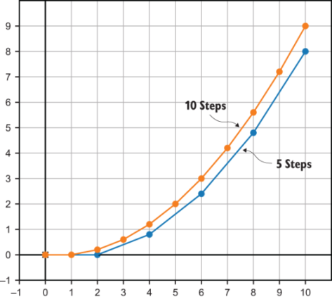
Figure 9.7 Euler’s method produces different results with the same initial values and different numbers of steps.

Trying again with 100 steps and dt = 0.1, we see yet another trajectory in the same 10 seconds (figure 9.8).

Figure 9.8 With 100 steps instead of 5 or 10, we get yet another trajectory. Dots are omitted for this trajectory because there are so many of them.

Why do we get different results even though the same equations went into all three calculations? It seems like the more time steps we use, the bigger the y-coordinates get. We can see the problem if we look closely at the first two seconds.

In the 5-step approximation, there’s no acceleration; the object is still traveling along the x-axis. In the 10-step approximation, the object has had one chance to update its velocity, so it has risen above the x-axis. Finally, the 100-step approximation has 19 velocity updates between t = 0 and t = 1, so its velocity increase is the largest (figure 9.9).

Figure 9.9 Looking closely at the first two segments, the 100-step approximation is the largest because its velocity updates most frequently.

This is what I swept under the rug earlier. The equation Δs = v · Δt is only correct when velocity is constant. Euler’s method is a good approximation when you use a lot of time steps because on smaller time intervals, velocity doesn’t change that much. To confirm this, you can try some large time steps with small values for dt. For example, with 100 steps of 0.1 seconds each, the final position is

(9.99999999999998, 9.900000000000006)

and with 100,000 steps of 0.0001 seconds each, the final position is

(9.999999999990033, 9.999899999993497)

The exact value of the final position is (10.0, 10.0), and as we add more and more steps to our approximation with Euler’s method, our results appear to converge to this value. You’ll have to trust me for now that (10.0, 10.0) is the exact value. We’ll cover how to do exact integrals in the next chapter to prove it. Stay tuned!

Exercises

def eulers_method(s0,v0,a,total_time,step_count):
    trajectory = [s0]
    s = s0
    v  = v0
    dt = total_time/step_count     ❶
    for _ in range(0,step_count):
        s = add(s,scale(dt,v))     ❷
        v  = add(v,scale(dt,a))
        trajectory.append(s)
    return trajectory

def eulers_method_overapprox(s0,v0,a,total_time,step_count):
    trajectory = [s0]
    s = s0
    v  = v0
    dt = total_time/step_count
    for _ in range(0,step_count):
        v  = add(v,scale(dt,a))
        s = add(s,scale(dt,v))
        trajectory.append(s)
    return trajectory

eulers_method_overapprox((0,0),(1,0),(0,0.2),10,10)
 

from math import pi,sin,cos
angle = 20 * pi/180
s0 = (0,1.5)
v0 = (30*cos(angle),30*sin(angle))
a = (0,−9.81)

result = eulers_method(s0,v0,a,3,100)

def baseball_trajectory(degrees):
    radians = degrees * pi/180
    s0 = (0,0)
    v0 = (30*cos(radians),30*sin(radians))
    a = (0,−9.81)
    return [(x,y) for (x,y) in eulers_method(s0,v0,a,10,1000) if y>=0]

from draw3d import *
traj3d = eulers_method((0,0,0), (1,2,0), (0,−1,1), 10, 10)
draw3d(
    Points3D(*traj3d)
)

>>> eulers_method((0,0,0), (1,2,0), (0,−1,1), 10, 1000)[−1]
(9.999999999999831, −29.949999999999644, 49.94999999999933)

Summary

• Velocity is the derivative of position with respect to time. It is a vector consisting of the derivatives of each of the position functions. In 2D, with position functions x(t) and y(t), we can write the position vector as a function s(t) = (x(t), y(t)) and the velocity vector as a function v(t) = (x'(t), y'(t)).

• In a video game, you can animate an object moving at a constant velocity by updating its position in each frame. Measuring the time between frames and multiplying it by the object’s velocity gives you the change in position for the frame.

• Acceleration is the derivative of velocity with respect to time. It is a vector whose components are the derivatives of the components of velocity, for instance, a(t) = (v'x(t), v'y(t)).

• To simulate an accelerating object in a video game, you need to not only update the position with each frame but also update the velocity.

• If you know the rate at which a quantity changes with respect to time, you can compute the value of a quantity itself over time by calculating the quantity’s change over many small time intervals. This is called Euler’s method.