This chapter covers

• Building and visualizing a simulation for a projectile
• Finding maximal and minimal values for a function using derivatives
• Tuning simulations with parameters
• Visualizing spaces of input parameters for simulations
• Implementing gradient ascent to maximize functions of several variables

For most of the last few chapters, we’ve focused on a physical simulation for a video game. This is a fun and simple example to work with, but there are far more important and lucrative applications. For any big feat of engineering like sending a rocket to Mars, building a bridge, or drilling an oil well, it’s important to know that it’s going to be safe, successful, and on budget before you attempt it. In each of these projects, there are quantities you want to optimize. For instance, you may want to minimize the travel time for your rocket, minimize the amount or cost of concrete in a bridge, or maximize the amount of oil produced by your well.

To learn about optimization, we’ll focus on the simple example of a projectile− namely, a cannonball being fired from a cannon. Assuming the cannonball comes out of the barrel at the same speed every time, the launch angle will decide the trajectory (figure 12.1).

Figure 12.1 Trajectories for a cannonball fired at four different launch angles

As you can see in figure 12.1, four different launch angles produce four different trajectories. Among these, 45° is the launch angle that sends the cannonball the furthest, while 80° is the angle that sends it the highest. These are only a few angles of all of the possible values between 0 and 90°, so we can’t be sure they are the best. Our goal is to systematically explore the range of possible launch angles to be sure we’ve found the one that optimizes the range of the cannon.

To do this, we first build a simulator for the cannonball. This simulator will be a Python function that takes a launch angle as input, runs Euler’s method (as we did in chapter 9) to simulate the moment-by-moment motion of the cannonball until it hits the ground, and outputs a list of positions of the cannonball over time. From the result, we’ll extract the final horizontal position of the cannonball, which will be the landing position or range. Putting these steps together, we implement a function that takes a launch angle and returns the range of the cannonball at that angle (figure 12.2).

Figure 12.2 Computing the range of a projectile using a simulator

Once we have encapsulated all of this logic in a single Python function called landing_position, which computes the range of a cannonball as a function of its launch angle, we can think about the problem of finding the launch angle that maximizes the range. We can do this in two ways: first, we make a graph of the range versus the launch angle and look for the largest value (figure 12.3).

Figure 12.3 Looking at a plot of range vs. launch angle, we can see the approximate value of the launch angle that produces the longest range.

The second way we can find the optimal launch angle is to set our simulator aside and find a formula for the range r(θ) of the projectile as a function of the launch angle θ. This should produce identical results as the simulation, but because it is a mathematical formula, we can take its derivative using the rules from chapter 10. The derivative of the landing position with respect to the launch angle tells us how much increase in the range we’ll get for small increases in the launch angle. At some angle, we can see that we get diminishing returns−increasing the launch angle causes the range to decrease and we’ll have passed our optimal value. Before this, the derivative of r(θ) will instantaneously be zero, and the value of θ where the derivative is zero happens to be the maximum value.

Once we’ve warmed up using both of these optimization techniques on our 2D simulation, we can try a more challenging 3D simulation, where we can control the upward angle of the cannon as well as the lateral direction it is fired. If the elevation of the terrain varies around the cannon, the direction can have an impact on how far the cannonball flies before hitting the ground (figure 12.4).

For this example, let’s build a function r(θ, φ), taking two input angles θ and φ and outputting a landing position. The challenge is to find the pair (θ, φ) that maximizes the range of the cannon. This example lets us cover our third and most important optimization technique: gradient ascent.

Figure 12.4 With uneven terrain, the direction we fire the cannon can affect the range of the cannonball as well.

As we learned in the last chapter, the gradient of r(θ, φ) at a point (θ, φ) is a vector pointing in the direction that causes r to increase most rapidly. We’ll write a Python function called gradient_ascent that takes as input a function to optimize, along with a pair of starting inputs, and uses the gradient to find higher and higher values until it reaches the optimal value.

The mathematical field of optimization is a broad one, and I hope to give you a sense of some basic techniques. All of the functions we’ll work with are smooth, so you will be able to make use of the many calculus tools you’ve learned so far. Also, the way we approach optimization in this chapter sets the stage for optimizing computer “intelligence” in machine learning algorithms, which we turn to in the final chapters of the book.

12.1 Testing a projectile simulation

Our first task is to build a simulator that computes the flight path of the cannonball. The simulator will be a Python function called trajectory. It takes the launch angle, as well as a few other parameters that we may want to control, and returns the positions of the cannonball over time until it collides with Earth. To build this simulation, we turn to our old friend from chapter 9−Euler’s method.

As a reminder, we can simulate motion with Euler’s method by advancing through time in small increments (we’ll use 0.01 seconds). At each moment, we’ll know the position of the cannonball, as well as its derivatives: velocity and acceleration. The velocity and acceleration let us approximate the change in position to the next moment, and we’ll repeat the process until the cannonball hits the ground. As we go, we can save the time, x and y positions of the cannonball, at each step and output them as the result of the trajectory function.

Finally, we’ll write functions that take the results we get back from the trajectory function and measure one numerical property. The functions landing _position, hang_time, and max_height tell us the range, the time in the air, and the maximum height of the cannonball, respectively. Each of these will be a value we can subsequently optimize for.

12.1.1 Building a simulation with Euler’s method

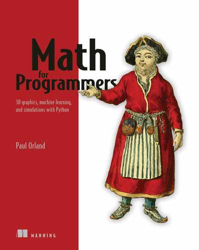
In our first 2D simulation, we call the horizontal direction the x direction and the vertical direction the z direction. That way we won’t have to rename either of these when we add another horizontal direction. We call the angle that the cannonball is launched θ and the velocity of the cannonball v as shown in figure 12.5.

Figure 12.5 The variables in our projectile simulation

The speed, v, of a moving object is defined as the magnitude of its velocity vector, so v = |v|. Given the launch angle θ, the x and z components of the cannonball’s velocity are v_x = |v| · cos(θ) and v_z = |v| · sin(θ). I’ll assume that the cannonball leaves the barrel of the cannon at time t = 0 and with (x, z) coordinates (0, 0), but I’ll also include a configurable launch height. Here’s the basic simulation using Euler’s method:

def trajectory(theta,speed=20,height=0,
               dt=0.01,g=−9.81):           ❶
    vx = speed * cos(pi * theta / 180)     ❷
    vz = speed * sin(pi * theta / 180)
    t,x,z = 0, 0, height
    ts, xs, zs = [t], [x], [z]             ❸
    while z >= 0:                          ❹
        t += dt                            ❺
        vz += g * dt
        x += vx * dt
        z += vz * dt
        ts.append(t)
        xs.append(x)
        zs.append(z)
    return ts, xs, zs                      ❻

❶ Additional inputs: the time step dt, gravitational field strength g, and angle theta (in degrees)

❷ Calculates the initial x and z components of velocity, converting the input angle from degrees to radians

❸ Initializes lists that hold all the values of time and the x and z positions over the course of the simulation

❹ Runs the simulation only while the cannonball is above ground

❺ Updates time, z velocity, and position. There are no forces acting in the x direction, so the x velocity is unchanged.

❻ Returns the list of t, x, and z values, giving the motion of the cannonball

You’ll find a plot_trajectories function in the source code for this book that takes the outputs of one or more results of the trajectory function and passes them to Matplotlib’s plot function, drawing curves that show the path of each cannonball. For instance, figure 12.6 shows plotting a 45° launch next to a 60° launch, which is done using the following code:

plot_trajectories( 
    trajectory(45),
    trajectory(60))

Figure 12.6 An output of the plot_trajectories function showing the results of a 45° and 60° launch angle.

We can already see that the 45° launch angle produces a greater range and that the 60° launch angle produces a greater maximum height. To be able to optimize these properties, we need to measure them from the trajectories.

12.1.2 Measuring properties of the trajectory

It’s useful to keep the raw output of the trajectory in case we want to plot it, but sometimes we’ll want to focus on one number that matters most. For instance, the range of the projectile is the last x-coordinate of the trajectory, which is the last x position before the cannonball hits the ground. Here’s a function that takes the result of the trajectory function (parallel lists with time and the x and z positions), and extracts the range or landing position. For the input trajectory, traj, traj[1] lists the x-coordinates, and traj[1][−1] is the last entry in the list:

def landing_position(traj):
    return traj[1][−1]

This is the main metric of a projectile’s trajectory that interests us, but we can also measure some other ones. For instance, we might want to know the hang time (or how long the cannonball stays in the air) or its maximum height. We can easily create other Python functions that measure these properties from simulated trajectories; for example,

def hang_time(traj):
    return traj[0][−1]   ❶
def max_height(traj):
    return max(traj[2])  ❷

❶ Total time in the air is equal to the last time value, the time on the clock when the projectile hits the ground.

❷ The maximum height is the maximum among the z positions, the third list in the trajectory output.

To find an optimal value for any of these metrics, we need to explore how the parameters (namely, the launch angle) affect them.

12.1.3 Exploring different launch angles

The trajectory function takes a launch angle and produces the full time and position data for the cannonball over its flight. A function like landing_position takes this data and produces a single number. Composing these two together (figure 12.7), we get a function for landing position in terms of the launch angle, where all other properties of the simulation are assumed constant.

Figure 12.7 Landing position as a function of the launch angle

One way to test the effect of the launch angle on a landing position is to make a plot of the resulting landing position for several different values of the launch angle (figure 12.8). To do this, we need to calculate the result of the composition landing_position (trajectory(theta)) for several different values of theta and pass these to Matplotlib’s scatter function. Here, for example, I use range(0,95,5) as the launch angles. This is every angle from zero to 90 in increments of 5:

import matplotlib.pyplot as plt
angles = range(0,90,5)
landing_positions = [landing_position(trajectory(theta)) 
                     for theta in angles]
plt.scatter(angles,landing_positions)

Figure 12.8 A plot of the landing position vs. the launch angle for the cannon for several different values of the launch angle

From this plot, we can guess what the optimal value is. At a launch angle of 45°, the landing position is maximized at a little over 40 meters from the launch position. In this case, 45° turns out to be the exact value of the angle that maximizes the landing position. In the next section, we’ll use calculus to confirm this maximum value without having to do any simulation.

12.1.4 Exercises

>>> landing_position(trajectory(50))
40.10994684444007
>>> landing_position(trajectory(130))
−40.10994684444007

def plot_trajectories(*trajs,show_seconds=False):
    for traj in trajs:
        xs, zs = traj[1], traj[2]
        plt.plot(xs,zs)
        if show_seconds:
            second_indices = []
            second = 0
            for i,t in enumerate(traj[0]):
                if t>= second:
                    second_indices.append(i)
                    second += 1
            plt.scatter([xs[i] for i in second_indices], 
                        [zs[i] for i in second_indices])
      ...

plot_trajectories(
    trajectory(20), 
    trajectory(45),
    trajectory(60),
    trajectory(80), 
    show_seconds=True)

test_angles = range(0,181,5)
hang_times = [hang_time(trajectory(theta)) for theta in test_angles]
plt.scatter(test_angles, hang_times)
 

plot_trajectory_metric(landing_position,[10,20,30]) 

plot_trajectory_metric(landing_position,[10,20,30], height=10)

def plot_trajectory_metric(metric,thetas,**settings):
    plt.scatter(thetas,
                [metric(trajectory(theta,**settings)) 
                 for theta in thetas])

plot_trajectory_metric(hang_time, range(0,181,5))

12.2 Calculating the optimal range

Using calculus, we can compute the maximum range for the cannon, as well as the launch angle that produces it. This actually takes two separate applications of calculus. First, we need to come up with an exact function that tells us the range r as a function of the launch angle θ. As a warning, this will take quite a bit of algebra. I’ll carefully walk you through all the steps, so don’t worry if you get lost; you’ll be able to jump ahead to the final form of the function r(θ) and continue reading.

Then I show you a trick using derivatives to find the maximum value of this function r(θ), and the angle θ that produces it. Namely, a value of θ that makes the derivative r'(θ) equal zero is also the value of θ that yields the maximum value of r(θ). It might not be immediately obvious why this works, but it will become clear once we examine the graph of r(θ) and study its changing slope.

12.2.1 Finding the projectile range as a function of the launch angle

The horizontal distance traveled by the cannonball is actually pretty simple to calculate. The x component of the velocity v_x is constant for its entire flight. For a flight of total time Δt, the projectile travels a total distance of r = v_x · Δt. The challenge is finding the exact value of that elapsed time Δt.

That time, in turn, depends on the z position of the projectile over time, which is a function z(t). Assuming the cannonball is launched from an initial height of zero, the first time that z(t) = 0 is when it’s launched at t = 0. The second time is the elapsed time we’re looking for. Figure 12.9 shows the graph of z(t) from the simulation with θ = 45°. Note that its shape looks a lot like the trajectory, but the horizontal axis (t) now represents time.

trj = trajectory(45)
ts, zs = trj[0], trj[2]
plt.plot(ts,zs)

Figure 12.9 A plot of z(t) for the projectile showing the launching and landing times where z = 0. We can see from the graph that the elapsed time is about 2.9 seconds.

We know z ''(t) = g = −9.81, which is the acceleration due to gravity. We also know the initial z velocity, z'(0) = |v| · sin(θ), and the initial z position, z(0) = 0. To recover the position function z(t), we need to integrate the acceleration z ''(t) twice. The first integral gives us velocity:

The second integral gives us position:

We can confirm that this formula matches the simulation by plotting it (figure 12.10). It is nearly indistinguishable from the simulation.

def z(t):                                         ❶
    return 20*sin(45*pi/180)*t + (−9.81/2)*t**2

plot_function(z,0,2.9)

❶ A direct translation of the result of the integral, z(t), into Python code

Figure 12.10 Plotting the exact function z(t) on top of the simulated values

For notational simplicity, let’s write the initial velocity |v| · sin(θ) as v_z so that z(t) = v_zt + gt²/2. We want to find the value of t that makes z(t) = 0, which is the total hang time for the cannonball. You may remember how to find that value from high school algebra, but if not, let me remind you quickly. If you want to know what value of t solves an equation at² + bt + c = 0, all you have to do is plug the values a, b, and c into the quadratic formula :

An equation like at² + bt + c = 0 can be satisfied twice; both times when our projectile hits z = 0. The symbol ± is shorthand to let you know that using a + or − at this point in the equation gives you two different (but valid) answers.

In the case of solving z(t) = v_zt + gt²/2 = 0, we have a = g/2, b = v_z and c = 0. Plugging into the formula, we find

Treating the ± symbol as a + (plus), the result is t = (− v_z + v_z)/g = 0. This says that z = 0 when t = 0, which is a good sanity check; it confirms that the cannonball starts at z = 0. The interesting solution is when we treat ± as a − (minus). In this case, the result is t = (− v_z − v_z)/g = −2v_z/g.

Let’s confirm the result makes sense. With an initial speed of 20 meters per second and a launch angle of 45° as we used in the simulation, the initial z velocity, v_z, is −2 · (20 · sin(45°))/−9.81 ¼ 2.88. This closely matches the result of 2.9 seconds that we read from the graph.

This gives us confidence in calculating the hang time Δt as Δt = −2v_z/g or Δt = −2|v|sin(θ)/g. Because the range is r = v_x · Δt = |v|cos(θ) · Δt, the full expression for the range r as a function of the launch angle θ is

We can plot this side by side with the simulated landing positions at various angles as in figure 12.11 and see that it agrees.

def r(theta):
    return (−2*20*20/−9.81)*sin(theta*pi/180)*cos(theta*pi/180)

plot_function(r,0,90)

Figure 12.11 Our calculation of projectile range as a function of the launch angle r(θ), which matches our simulated landing positions

Having a function r(θ) is a big advantage over repeatedly running the simulator. First of all, it tells us the range of the cannon at every launch angle, not just a handful of angles that we simulated. Second, it is much less computationally expensive to evaluate this one function than to run hundreds of iterations of Euler’s method. For more complicated simulations, this could make a big difference. Additionally, this function gives us the exact result rather than an approximation. The final benefit, which we’ll make use of next, is that the function r(θ) is smooth, so we can take its derivatives. This gives us an understanding of how the range of the projectile changes with respect to the launch angle.

12.2.2 Solving for the maximum range

Looking at the graph of r(θ) in figure 12.12, we can set our expectations for what the derivative r'(θ) will look like. As we increase the launch angle from zero, the range increases as well for a while but at a decreasing rate. Eventually, increasing the launch angle begins to decrease the range.

The key observation to make is that while r'(θ) is positive, the range is increasing with respect to θ. Then the derivative r'(θ) crosses below zero, and the range decreases from there. It is precisely at this angle (where the derivative is zero) that the function r(θ) achieves its maximum value. You can visualize this by seeing that the graph of r(θ) in figure 12.12 hits its maximum when the slope of the graph is zero.

Figure 12.12 The graph of r(θ) hits its maximum when the derivative is zero and, therefore, the slope of the graph is zero.

We should be able to take the derivative of r(θ) symbolically, find where it equals zero between 0° and 90°, and this should agree with the rough maximum value of 45°. Remember that the formula for r is

Because −2|v|²/g is constant with respect to θ, the only hard work is using the product rule on sin(θ)cos(θ). The result is

Notice that I factored out the minus sign. If you haven’t seen this notation before, sin²(θ) means (sin(θ))². The value of the derivative r'(θ) is zero when the expression sin²(θ) − cos²(θ) is zero (in other words, we can ignore the constants). There are a few ways to figure out where this expression is zero, but a particularly nice one is to use the trigonometric identity, cos(2θ) = cos²(θ) − sin²(θ), which reduces our problem even further. Now we need to figure out where cos(2θ) = 0.

The cosine function is zero at π/2 plus any multiple of π, or 90° plus any multiple of 180° (that is, 90°, 270°, 430°, and so on). If 2θ is equal to these values, θ could be half of any of these values: 45°, 135°, 215°, and so on.

Of these, there are two interesting results. First, θ = 45° is the solution between θ = 0 and θ = 90°, so it is both the solution we expected and the solution we’re looking for! The second interesting solution is 135° because this is the same as shooting the cannonball at 45° in the opposite direction (figure 12.13).

Figure 12.13 In our model, shooting the cannonball at 135° is like shooting at 45° in the opposite direction.

At angles of 45° and 135°, the resulting ranges are

>>> r(45)
40.774719673802245
>>> r(135)
−40.77471967380224

It turns out that these are the extremes of where the cannonball can end up, with all other parameters equal. A launch angle of 45° produces the maximum landing position, while a launch angle of 135° produces the minimum landing position.

12.2.3 Identifying maxima and minima

To see the difference between the maximum range at 45° and the minimum range at 135°, we can extend the plot of r(θ). Remember, we found both of these angles because they were at places where the derivative r'(θ) was zero (figure 12.14).

Figure 12.14 The angles θ = 45° and θ = 135° are the two values between 0 and 180 where r'(θ) = 0.

While maxima(the plural of “maximum”) of smooth functions occur where the derivative is zero, the converse is not always true; not every place where the derivative is zero yields a maximum value. As we see in figure 12.14 at θ = 135°, it can also yield a minimum value of a function.

You need to be cautious of the global behavior of functions as well, because the derivative can be zero at what’s called a local maximum or minimum, where the function briefly obtains a maximum or minimum value, but it’s real, global maximum or minimum values lie elsewhere. Figure 12.15 shows a classic example: y = x³ − x. Zooming in on the region where −1 < x < 1, there are two places where the derivative is zero, which look like a maximum and minimum, respectively. When you zoom out, you see that neither of these is the maximum or minimum value for the whole function because it goes off to infinity in both directions.

Figure 12.15 Two points that are a local minimum and local maximum, but neither is the minimum or maximum value for the function

As another confounding possibility, a point where the derivative is zero may not even be a local minimum or maximum. For instance, the function y = x³ has a derivative of zero at x = 0 (figure 12.16). This point just happens to be a place where the function x³ stops increasing momentarily.

Figure 12.16 For y = x³, the derivative is zero at x = 0, but this is not a minimum or maximum value.

I won’t go into the technicalities of telling whether a point with a zero derivative is a minimum, maximum, or neither, or how to distinguish local minima and maxima from global ones. The key idea is that you need to fully understand the behavior of a function before you can confidently say you’ve found an optimal value. With this in mind, let’s move on to some more complicated functions to optimize and some new techniques for optimizing them.

12.2.4 Exercises

12.3 Enhancing our simulation

As your simulator becomes more complicated, there can be multiple parameters governing its behavior. For our original cannon, the launch angle θ was the only parameter we were playing with. To optimize the range of the cannon, we worked with a function of one variable: r(θ). In this section, we’ll make our cannon fire in 3D, meaning that we need to vary two launch angles as parameters to optimize the range of the cannonball.

12.3.1 Adding another dimension

The first thing is to add a y dimension to our simulation. We can now picture the cannon sitting at the origin of the x,y plane, shooting the cannonball up into the z direction at some angle θ. In this version of the simulator, you can control the angle θ as well as a second angle, which we’ll call φ (the Greek letter phi). This measures how far the cannon is rotated laterally from the +x direction (figure 12.17).

Figure 12.17 Picturing the cannon firing in 3D. Two angles θ and ϕ determine the direction the cannon is fired.

To simulate the cannon in 3D, we need to add motion in the y direction. The physics in the z direction remains exactly the same, but the horizontal velocity is split between the x and y direction, depending on the value of the angle φ. Whereas the previous x component of the initial velocity was v_x = |v|cos(θ), it’s now scaled by a factor of cos(φ) to give v_x = |v|cos(θ)cos(φ). The y component of initial velocity is v_y = |v|cos(θ)sin(φ). Because gravity doesn’t act in the y direction, we don’t have to update v_y over the course of the simulation. Here’s the updated trajectory function:

def trajectory3d(theta,phi,speed=20,
                 height=0,dt=0.01,g=−9.81):          ❶
    vx = speed * cos(pi*theta/180)*cos(pi*phi/180)
    vy = speed * cos(pi*theta/180)*sin(pi*phi/180)   ❷
    vz = speed * sin(pi*theta/180)
    t,x,y,z = 0, 0, 0, height
    ts, xs, ys, zs = [t], [x], [y], [z]              ❸
    while z >= 0:
        t += dt
        vz += g * dt
        x += vx * dt
        y += vy * dt                                 ❹
        z += vz * dt
        ts.append(t)
        xs.append(x)
        ys.append(y)
        zs.append(z)
    return ts, xs, ys, zs

❶ The lateral angle ϕ is the input parameter of the simulation.

❷ Calculates the initial y velocity

❸ Stores the values of time and the x, y, and z positions throughout the simulation

❹ Updates the y position in each iteration

If this simulation is successful, we don’t expect it to change the angle θ that yields the maximum range. Whether you fire a projectile at 45° above the horizontal in the +x direction, the − x direction, or any other direction in the plane, the projectile should go the same distance. That is to say that φ doesn’t affect the distance traveled. Next, we add the terrain with a variable elevation around the launch point so the distance traveled changes.

12.3.2 Modeling terrain around the cannon

Hills and valleys around the cannon mean that its shots can stay in the air for different durations depending on where they’re aimed. We can model the elevation above or below the plane z = 0 by a function that returns a number for every (x,y) point. For instance,

def flat_ground(x,y):
    return 0

represents flat ground, where the elevation at every (x,y) point is zero. Another function we’ll use is a ridge between two valleys:

def ridge(x,y):
    return (x**2 − 5*y**2) / 2500

On this ridge, the ground slopes upward from the origin in the positive and negative x directions, and it slopes downward in the positive and negative y directions. (You can plot the cross sections of this function at x = 0 and y = 0 to confirm this.)

Whether we want to simulate the projectile on flat ground or on the ridge, we have to adapt the trajectory3d function to terminate when the projectile hits the ground, not just when its altitude is zero. To do this, we can pass the elevation function defining the terrain as a keyword argument, defaulting to flat ground, and revise the test for whether the projectile is above ground. Here are the changed lines in the function:

def trajectory3d(theta,phi,speed=20,height=0,dt=0.01,g=−9.81,
                    elevation=flat_ground):
    ...
    while z >= elevation(x,y):
       ...

In the source code, I also provide a function called plot_trajectories_3d, which plots the result of trajectory3D as well as the specified terrain. To confirm our simulation works, we see the trajectory end below z = 0 when the cannonball is fired downhill and above z = 0 when it is fired uphill (figure 12.18):

plot_trajectories_3d(
    trajectory3d(20,0,elevation=ridge),
    trajectory3d(20,270,elevation=ridge),
    bounds=[0,40,−40,0],
    elevation=ridge)

Figure 12.18 A projectile fired downhill lands below z = 0 and a projectile fired uphill lands above z = 0.

If you had to guess, it seems reasonable that the maximum range for the cannon is attained in the downhill direction rather than the uphill direction. On its way down, the cannonball has further to fall, taking more time and allowing it to travel further. It’s not clear if the vertical angle θ will yield the optimal range because our calculation of 45° made the assumption that the ground was flat. To answer this question, we need to write the range r of the projectile as a function of θ and φ.

12.3.3 Solving for the range of the projectile in 3D

Even though the cannonball is fired in 3D space in our latest simulation, its trajectory lies in a vertical plane. As such, given an angle φ, we only need to work with the slice of the terrain in the direction the cannonball is fired. For instance, if the cannonball is fired at an angle φ = 240°, we only need to think about terrain values when (x, y) lies along a line at 240° from the origin. This is like thinking about the elevation of the terrain only at the points in the shadow cast by the trajectory (figure 12.19).

Figure 12.19 We only need to think about the elevation of the terrain in the plane where the projectile is fired. This is where the shadow of the trajectory is cast.

Our goal is to do all of our calculations in the plane of the shadow’s trajectory, working with the distance d from the origin in the x,y plane as our coordinate, rather than x and y themselves. At some distance, the trajectory of the cannonball and the elevation of the terrain will have the same z value, which is where the cannonball stops. This distance is the range that we want to find an expression for.

Let’s keep calling the height of the projectile z. As a function of time, the height is exactly the same as in our 2D example

where v_z is the z component of the initial velocity. The x and y positions are also given as simple functions of time x(t) = v_xt and y(t) = v_yt because no forces act in the x or y direction.

On the ridge, the elevation is given as a function of the x, y position by (x² − 5y²)/2500. We can write this elevation as h(x, y) = B_x² − C_y² where B = 1/2500 = 0.0004 and C = 5/2500 = 0.002. It’s useful to know the elevation of the terrain directly under the projectile at a given time t, which we can call h(t). We can calculate the value of h under the projectile at any point in time t because the projectile’s x and y positions are given by v_xt and v_yt, and the elevation at the same (x, y) point will be h(v_xt, v_yt) = Bv_x² t² − Cv_y² t².

The altitude of the projectile above the ground at a time t is the difference between z(t) and h(t). The time of impact is the time when this difference is zero, that is z(t) − h(t) = 0. We can expand that condition in terms of the definitions of z(t) and h(t):

Once again, we can reshape this into the form at² + bt + c = 0:

Specifically, a = g/2 − Bv_x² + Cv_y², b = v_z and c = 0. To find the time t that satisfies this equation, we can use the quadratic formula:

Because c = 0, the form is even simpler:

When we use the + operator, we find t = 0, confirming that the cannonball is at ground level at the moment it is launched. The interesting solution is obtained using the − operator, which is the time the projectile lands. This time is t = (− b − b)/2a = − b/a. Plugging in the expressions for a and b, we get an expression for landing time in terms of quantities we know how to calculate:

The distance in the (x,y) plane that the projectile lands is for this time t. That expands to . You can think of as the component of the initial velocity parallel to the x,y plane, so I’ll call this number vxy. The distance at landing is

All of these numbers in the expression are either constants that I specified or are computed in terms of the initial speed v = |v| and the launch angles θ and φ. It’s straightforward (albeit a bit tedious) to translate this to Python, where it becomes clear exactly how we can view the distance as a function of θ and φ:

B = 0.0004                                         ❶
C = 0.005
v = 20
g = −9.81

def velocity_components(v,theta,phi):              ❷
    vx = v  * cos(theta*pi/180) * cos(phi*pi/180)
    vy = v  * cos(theta*pi/180) * sin(phi*pi/180)
    vz = v  * sin(theta*pi/180)
    return vx,vy,vz
    
def landing_distance(theta,phi):
    vx, vy, vz = velocity_components(v, theta, phi)
    v_xy = sqrt(vx**2 + vy**2)                     ❸
    a = (g/2) − B * vx**2 + C * vy**2              ❹
    b = vz
    landing_time = -b/a                            ❺
    landing_distance = v_xy * landing_time         ❻
    return landing_distance

❶ Constants for the shape of the ridge, launch speed, and acceleration due to gravity

❷ A helper function that finds the x, y, and z components of the initial velocity

❸ The horizontal component of initial velocity (parallel to the x,y plane)

❹ The constants a and b

❺ Solves the quadratic equation for landing time, which is -b/a

❻ The horizontal distance traveled

The horizontal distance traveled is the horizontal velocity times the elapsed time. Plotting this point alongside the simulated trajectory, we can verify that our calculated value for the landing position matches the simulation with Euler’s method (figure 12.20).

Figure 12.20 Comparing the calculated landing point with the result of the simulation for θ = 30° and ϕ = 240°

Now that we have a function r(θ, φ) for the range of the cannon in terms of the launch angles θ and φ, we can turn our attention to finding the angles that optimize the range.

12.3.4 Exercises

def trajectory3d(theta,phi,speed=20,height=0,dt=0.01,g=−9.81,
                 elevation=flat_ground, drag=0):
    ...
    while z >= elevation(x,y):
        t += dt
        vx -= (drag * vx) * dt         ❶
        vy -= (drag * vy) * dt
        vz += (g − (drag * vz)) * dt   ❷
        ...
    return ts, xs, ys, zs

12.4 Optimizing range using gradient ascent

Let’s continue to assume that we’re firing the cannon on the ridge terrain with some launch angles θ and φ, and all other launch parameters set to their defaults. In this case, the function r(θ, φ) tells us what the range of the cannon is at these launch angles. To get a qualitative sense of how the angles affect the range, we can plot the function r .

12.4.1 Plotting range versus launch parameters

I showed you a few different ways to plot a function of two variables in the last chapter. My preference for plotting r(θ, φ) is to use a heatmap. On a 2D canvas, we can vary θ in one direction and vary φ in the other and then use color to indicate the corresponding range of the projectile (figure 12.21).

Figure 12.21 A heatmap of the range of the cannon as a function of the launch angles θ and ϕ

This 2D space is an abstract one, having coordinates θ and φ. That is to say that this rectangle isn’t a drawing of a 2D slice of the 3D world we’ve modelled. Rather, it’s just a convenient way to show how the range r varies as the two parameters change.

On the graph in figure 12.22, brighter values indicate higher ranges, and there appear to be two brightest points. These are possible maximum values of the range of the cannon.

Figure 12.22 The brightest spots occur when the range of the projectile is maximized.

These spots occur at around θ = 40, φ = 90, and φ = 270. The φ values make sense because they are the downhill directions in the ridge. Our next goal is to find the exact values of θ and φ to maximize the range.

12.4.2 The gradient of the range function

Just as we used the derivative of a function of one variable to find its maximum, we’ll use the gradient ∇r(θ, φ) of the function r(θ, φ) to find its maximum values. For a smooth function of one variable, f(x), we saw that f'(x) = 0 when f attained its maximum value. This is when the graph of f(x) was momentarily flat, meaning the slope of f(x) was zero, or more precisely, that the slope of the line of best approximation at the given point was zero. Similarly, if we make a 3D plot of r(θ, φ), we can see that it is flat at its maximum points (figure 12.23).

Figure 12.23 The graph of r(θ, ϕ) is flat at its maximum points.

Let’s be precise about what this means. Because r(θ, φ) is smooth, there is a plane of best approximation. The slopes of this plane in the θ and φ directions are given by the partial derivatives ∂r/∂θ and ∂r/∂φ, respectively. Only when both of these are zero is the plane flat, meaning the graph of r(θ, φ) is flat.

Because the partial derivatives of r are defined to be the components of the gradient of r , this condition of flatness is equivalent to saying that ∇r(θ, φ) = 0. To find such points, we have to take the gradient of the full formula for r(θ, φ) and then solve for values of θ and φ that cause it to be zero. Taking these derivatives and solving them is a lot of work and not that enlightening, so I’ll leave it as an exercise for you. Next, I’ll show you a way to follow an approximate gradient up the slope of the graph toward the maximum point, which won’t require any algebra.

Before I move on, I want to reiterate a point from the previous section. Just because you’ve found a point on the graph where the gradient is zero doesn’t mean that it’s a maximum value. For instance, on the graph of r(θ, φ), there’s a point in between the two maxima where the graph is flat and the gradient is zero (figure 12.24).

Figure 12.24 A point (θ, ϕ) where the graph of r(θ, ϕ) is flat. The gradient is zero, but the function does not attain a maximum value.

This point isn’t meaningless, it happens to tell you the best angle θ when you’re shooting the projectile at φ = 180°, which is the worst possible direction because it is the steepest uphill direction. A point like this is called a saddle point, where the function simultaneously hits a maximum with respect to one variable and a minimum with respect to another. The name comes from the fact that the graph kind of looks like a saddle.

Again, I won’t go into the details of how to identify maxima, minima, saddle points, or other kinds of places where the gradient is zero, but be warned: with more dimensions, there are weirder ways that a graph can be flat.

12.4.3 Finding the uphill direction with the gradient

Rather than take the partial derivatives of the complicated function r(θ, φ) symbolically, we can find approximate values for the partial derivatives. The direction of the gradient that they give us tells us, for any given point, which direction the function increases the most quickly. If we jump to a new point in this direction, we should move uphill and towards a maximum value. This procedure is called gradient ascent, and we’ll implement it in Python.

The first step is to be able to approximate the gradient at any point. To do that, we use the approach I introduced in chapter 9: taking the slopes of small secant lines. Here are the functions as a reminder:

def secant_slope(f,xmin,xmax):                ❶
    return (f(xmax) − f(xmin)) / (xmax − xmin)

def approx_derivative(f,x,dx=1e−6):           ❷
    return secant_slope(f,x-dx,x+dx)

❶ Finds the slope of a secant line, f(x), between x values of xmin and xmax

❷ The approximate derivative is a secant line between x − 10 − 6 and x + 10 − 6.

To find the approximate partial derivative of a function f(x, y) at a point (x₀, y₀), we want to fix x = x₀ and take the derivative with respect to y, or fix y = y₀ and take the derivative with respect to x. In other words, the partial derivative ∂f/∂x at (x₀, y₀) is the ordinary derivative of f(x, y₀) with respect to x at x = x₀. Likewise, the partial derivative ∂f/∂y is the ordinary derivative of f(x₀, y) with respect to y at y = y₀. The gradient is a vector (tuple) of these partial derivatives:

def approx_gradient(f,x0,y0,dx=1e−6):
    partial_x = approx_derivative(lambda x: f(x,y0), x0, dx=dx)
    partial_y = approx_derivative(lambda y: f(x0,y), y0, dx=dx)
    return (partial_x,partial_y)

In Python, the function r(θ, φ) is encoded as the landing_distance function, and we can store a special function, approx_gradient, representing its gradient:

def landing_distance_gradient(theta,phi):
    return approx_gradient(landing_distance_gradient, theta, phi)

This, like all gradients, defines a vector field: an assignment of a vector to every point in space. In this case, it tells us the vector of steepest increase in r at any point (θ, φ). Figure 12.25 shows the plot of the landing_distance_gradient on top of the heatmap for r(θ, φ).

Figure 12.25 A plot of the gradient vector field ∇r(θ, ϕ) on top of the heatmap of the function r(θ, ϕ). The arrows point in the direction of increase in r, toward brighter spots on the heatmap.

It’s even clearer that the gradient arrows converge on maximum points for the function if you zoom in (figure 12.26).

Figure 12.26 The same plot as in figure 12.25 near (θ, ϕ) = (37.5°, 90°), which is the approximate location of one of the maxima

The next step is to implement the gradient ascent algorithm, where we start at an arbitrarily chosen point (θ, φ) and follow the gradient field until we arrive at a maximum.

12.4.4 Implementing gradient ascent

The gradient ascent algorithm takes as inputs the function we’re trying to maximize, as well as a starting point where we’ll begin our exploration. Our simple implementation calculates the gradient at the starting point and adds it to the starting point, giving us a new point some distance away from the original in the direction of the gradient. Repeating this process, we can move to points closer and closer to a maximum value.

Eventually, as we approach a maximum, the gradient will get close to zero as the graph reaches a plateau. When the gradient is near zero, we have nowhere further uphill to go, and the algorithm should terminate. To make this happen, we can pass in a tolerance, which is the smallest value of the gradient that we should follow. If the gradient is smaller, we can be assured the graph is flat, and we’ve arrived at a maximum for the function. Here’s the implementation:

def gradient_ascent(f,xstart,ystart,tolerance=1e−6):
    x = xstart                                       ❶
    y = ystart
    grad = approx_gradient(f,x,y)                    ❷
    while length(grad) > tolerance:                  ❸
        x += grad[0]                                 ❹
        y += grad[1]
        grad = approx_gradient(f,x,y)                ❺
    return x,y                                       ❻

❶ Sets the initial values of (x, y) to the input values

❷ Tells us how to move uphill from the current (x, y) value

❸ Only steps to a new point if the gradient is longer than the minimum length

❹ Updates (x, y) to (x, y) + ∇f(x, y)

❺ Updates the gradient at this new point

❻ When there’s nowhere further uphill to go, returns the values of x and y

Let’s test this, starting at the value of (θ, φ) = (36°, 83°), which appears to be fairly close to the maximum:

>>> gradient_ascent(landing_distance,36,83)
(37.58114751557887, 89.99992616039857)

This is a promising result! On our heatmap in figure 12.27, we can see the movement from the initial point of (θ, φ) = (36°, 83°) to a new location of roughly (θ, φ) = (37.58, 90.00), which looks like it has the maximum brightness.

Figure 12.27 The starting and ending points for the gradient ascent

To get a better sense of how the algorithm works, we can track the trajectory of the gradient ascent through the θ, φ plane. This is similar to how we tracked the time and position values as we iterated through Euler’s method:

def gradient_ascent_points(f,xstart,ystart,tolerance=1e−6):
    x = xstart
    y = ystart
    xs, ys = [x], [y]
    grad = approx_gradient(f,x,y)
    while length(grad) > tolerance:
        x += grad[0]
        y += grad[1]
        grad = approx_gradient(f,x,y)
        xs.append(x)
        ys.append(y)
    return xs, ys

With this implemented, we can run

gradient_ascent_points(landing_distance,36,83)

and we get back two lists, consisting of the θ values and the φ values at each step of the ascent. These lists both have 855 numbers, meaning that this gradient ascent took 855 steps to complete. When we plot the θ and φ points on the heatmap (figure 12.28), we can see the path that our algorithm took to ascend the graph.

Figure 12.28 The path that the gradient ascent algorithm takes to reach the maximum value of the range function

Note that because there are two maximum values, the path and the destination depend on our choice of the initial point. If we start close to φ = 90°, we’re likely to hit that maximum, but if we’re closer to φ = 270°, our algorithm finds that one instead (figure 12.29).

Figure 12.29 Starting at different points, the gradient ascent algorithm can find different maximum values.

The launch angles (37.58°, 90°) and (37.58°, 270°) both maximize the function r(θ, φ) and are, therefore, the launch angles that yield the greatest range for the cannon. That range is about 53 meters

>>> landing_distance(37.58114751557887, 89.99992616039857)
52.98310689354378

and we can plot the associated trajectories as shown in figure 12.30.

Figure 12.30 The trajectories for the cannon having maximum range

As we explore some machine learning applications, we’ll continue to rely on the gradient to figure out how to optimize functions. Specifically, we’ll use the counterpart to gradient ascent, called gradient descent. This finds the minimum values for functions by exploring the parameter space in the direction opposite the gradient, thereby moving downhill instead of uphill. Because gradient ascent and descent can be performed automatically, we’ll see they give a way for machines to learn optimal solutions to problems on their own.

12.4.5 Exercises

from random import uniform
for x in range(0,20):
    gap = gradient_ascent_points(landing_distance, 
                                 uniform(0,90), 
                                 uniform(0,360))
    plt.plot(*gap,c='k')

>>> gradient_ascent(landing_distance,0,180)
(46.122613357930206, 180.0)

def gradient_ascent_points(f,xstart,ystart,rate=1,tolerance=1e−6):
    ...
    while length(grad) > tolerance:
        x += rate * grad[0]
        y += rate * grad[1]
        ...
    return xs, ys

def count_ascent_steps(f,x,y,rate=1):
    gap = gradient_ascent_points(f,x,y,rate=rate)
    print(gap[0][−1],gap[1][−1])
    return len(gap[0])

>>> count_ascent_steps(landing_distance,36,83)
855

>>> count_ascent_steps(landing_distance,36,83,rate=1.5)
568

>>> count_ascent_steps(landing_distance,36,83,rate=3)
282
>>> count_ascent_steps(landing_distance,36,83,rate=10)
81
>>> count_ascent_steps(landing_distance,36,83,rate=20)
38

Summary

• We can simulate a moving object’s trajectory by using Euler’s method and recording all of the times and positions along the way. We can compute facts about the trajectory, like final position or elapsed time.

• Varying a parameter of our simulation, like the launch angle of the cannon, can lead to different results−for instance, a different range for the cannonball. If we want to find the angle that maximizes range, it helps to write range as a function of the angle r(θ).

• Maximum values of a smooth function f(x) occur where the derivative f'(x) is zero. You need to be careful, though, because when f'(x) = 0, the function f might be at a maximum value, or it could also be a minimum value or a point where function f has temporarily stopped changing.

• To optimize a function of two variables, like the range r as a function of the vertical launch angle θ and the lateral launch angle φ, you need to explore the 2D space of all possible inputs (θ, φ) and figure out which pair produces the optimal value.

• Maximum and minimum values of a smooth function of two variables f(x, y) occur when both partial derivatives are zero; that is, ∂f/∂x = 0 and ∂f/∂y = 0, so ∇f(x, y) = 0 as well (by definition). If the partial derivatives are zero, it might also be a saddle point, which minimizes the function with respect to one variable while maximizing it with respect to the other.

• The gradient ascent algorithm finds an approximate maximum value for a function f(x,y) by starting at an arbitrarily chosen point in 2D and moving in the direction of the gradient ∇f(x, y). Because the gradient points in the direction of most rapid increase in the function f , this algorithm finds (x, y) points with increasing f values. The algorithm terminates when the gradient is near zero.