
3
A Survey of Classification Techniques in Speech Emotion Recognition
Tanmoy Roy1, Tshilidzi Marwala1, and Snehashish Chakraverty2
1Electrical and Electronic Engineering Science, University of Johannesburg, Johannesburg, 2006, South Africa
2Department of Mathematics, National Institute of Technology, Rourkela, Odisha, 769008, India
3.1 Introduction
Speech recognition models are presently in a very advanced state, and examples such as Siri, Cortana, and Alexa are the technical marvels that not can only hear us comfortably, but those bots can reply to us with equal comfort as well. However, speech recognition systems cannot detect the underlying emotion in speech signals. Speech emotion recognition (SER) is the field of study that explores the avenues of detecting emotions concealed in speech signals. The initial study on emotion started as a study of psychology and acoustics of emotions. The first detailed study on emotions was reported way back in 1872 by Charles Darwin [1]. Fairbanks and Pronovost [2] were among the first who studied pitch of voice during simulated emotion. Since the late 1950s, there has been a significant increase in interest by researchers regarding the psychological and acoustic aspects of emotion [3–6]. However, in the year 1995, Picard [7] introduced the term “affective computing,” and after that, the study of emotional states has become an integral part of artificial intelligence (AI) research.
SER is a machine learning (ML) problem where the speech utterances are classified depending on their underlying emotions. This chapter gives an overview of the prominent classification techniques used in SER. Researchers used different types of classifiers for SER, but in most of the situations, a proper justification is not provided for choosing a particular classification model [8]. Two plausible explanations are that classifiers that are successful in automatic speech recognition (ASR) are assumed to be working well in SER (like hidden Markov model [HMM]), and secondly, those classifiers that perform well in most classification problems are chosen [9]. There are two broad categories of classifiers (Figure 3.1) used in SER: the linear classifiers and the non‐linear classifiers. Although many classification models have been used for SER, but few among them become effective and popular among the researchers. Four classification models, namely HMM, Gaussian mixture model (GMM), support vector machine (SVM), and deep learning (DL), have been identified as prominent for this work and they are discussed in Sections 3.4.1–3.4.4.
3.2 Emotional Speech Databases
Researchers are trying to solve SER as an ML problem, and ML approaches are data‐driven. Moreover, SER research field is not mature enough to identify the underlying emotion of a random spoken conversion. Thus, the SER research depends heavily on emotional speech databases [10,11]. The speech databases created by researchers and organizations to support the SER research. The database naturalness, quality of recordings, number and type of emotions considered, and speech collection strategy are critical inputs for the classification stage because those features of the database will decide the classification methodology [12–15]. The design of the speech database can have different factors [13,16]. First of all, the existing databases can be categorized into three categories: (i) simulated by actors, (ii) seminatural, and (iii) natural. The simulated databases, created by enacting emotions by actors, are usually well annotated, adequately labeled, and are of better quality because the recordings are performed in a controlled near noise‐free environment. The number of recordings is also usually high for simulated databases. However, acted emotions are not natural enough, and sometimes, an expression of the same emotion varies a lot depending on the actor, which makes the feature selection process very difficult. Seminatural databases are also the collection of the enactions by professional or nonprofessional actors, but here, the actors are trying to keep it as natural as possible. Natural emotional databases are difficult to label because manually labeling a big set of speech recordings is a daunting task, and there is no method available yet to label the emotions automatically. As a result, the number of emotions covered in a natural dataset is low, and the number of data points is also low. Natural recordings usually depict continuous emotions, which can create hurdles during the classification phase because of the presence of overlapping emotions.
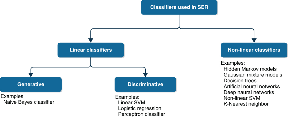
Figure 3.1 Categories of classifiers used in SER along with some examples.
3.3 SER Features
Feature selection and feature extraction are vital steps toward building a successful classification model. In SER, various types of features are extracted from the speech signals. Speech signals carry an enormous amount of information apart from the intended message. Researchers agreed that speech signals also carry vital information regarding the emotional state of the speaker [17]. However, researchers are still undecided over the right set of features of the speech signals, which can represent the underlying emotional state. This section contains the details of feature sets that are heavily used so far in SER research and performed well in the classification stage. There are three prominent categories in speech features used in SER: (i) the prosodic features, (ii) the spectral or vocal tract features, and (iii) the excitation source features.
Prosody features are the characteristics of the speech sound generated by the human speech production system, for example, pitch or fundamental frequency (![]() ) and energy. Researchers used different derivatives of pitch and energy as various prosody features [18–20]. These are also called continuous features and can be grouped into the following categories [8,16,21,22]: (i) pitch‐related features, (ii) formant features, (iii) energy‐related features, (iv) timing features, and (v) articulation features. Several studies tried to establish the relationship between prosody speech features and the underlying patterns of different emotions [21–28].
) and energy. Researchers used different derivatives of pitch and energy as various prosody features [18–20]. These are also called continuous features and can be grouped into the following categories [8,16,21,22]: (i) pitch‐related features, (ii) formant features, (iii) energy‐related features, (iv) timing features, and (v) articulation features. Several studies tried to establish the relationship between prosody speech features and the underlying patterns of different emotions [21–28].
The features used to represent glottal activity, mainly the vibration of glottal folds, are known as the source or excitation source features. These are also called voice quality features because glottal folds determine the characteristics of the voice. Some researchers believed that the emotional content of an utterance is strongly related to voice quality [21,29,30]. Voice quality measures for a speech signal includes harshness, breathiness, and tenseness. The relation of voice quality features with different emotions is not a well‐explored area, and researchers have produced contradictory conclusions. For example, Scherer [29] associated anger with tense voice, whereas Murray and Arnott [22] associated anger with a breathy voice.
Spectral features are the characteristics of various sound components generated from different cavities of the vocal tract system. They are also called segmental or system features. Spectral features extracted in the form of
- ordinary linear predictor coefficients (LPC) [31],
- one‐sided autocorrelation linear predictor coefficients (OSALPC) [32],
- short‐time coherence method (SMC) [33], and
- least‐squares modified Yule–Walker equations (LSMYWE) [34].
There is a particular type of spectral feature called the cepstral features, which are extensively used by SER researchers. Cepstral features can be derived from the corresponding linear features such as linear predictor cepstral coefficients (LPCC) is derived from linear predictor (LP). Mel‐frequency cepstral coefficients are one such cepstral feature that along with its various derivatives is widely used in SER research [35–39].
3.4 Classification Techniques
SER deals with speech signals. The analog (continuous) speech signal is sampled at a specified time interval to get the discrete time speech signal. A discrete time signal can be represented as follows:

where ![]() is the total number of sample points in the speech signal. First, only the speech utterance section is extracted from the speech sound by using a speech endpoint detection algorithm. In this case, an algorithm proposed by Roy et al. [40] is used.
is the total number of sample points in the speech signal. First, only the speech utterance section is extracted from the speech sound by using a speech endpoint detection algorithm. In this case, an algorithm proposed by Roy et al. [40] is used.
This speech signal contains various information that can be retrieved for further processing. Emotional states guide human thoughts, and those thoughts are expressed in different forms [41], such as speech. The primary objective of an SER is to find the patterns in speech signals, which can describe the underlying emotions. The pattern recognition task is carried out by different ML algorithms. Features are extracted from the speech signal ![]() in two forms
in two forms
- local features by splitting the signals into smaller frames and computing statistics of each frame and
- global features by calculating statistics on the whole utterance.
Let, there be ![]() number of sample points after the feature extraction process. If local features are computed from
number of sample points after the feature extraction process. If local features are computed from ![]() by assuming 10 splits, then there will be 10 data points from
by assuming 10 splits, then there will be 10 data points from ![]() . Now, suppose there is a total of 100 recorded utterances, and each utterance is split into 10 frames, then will be total
. Now, suppose there is a total of 100 recorded utterances, and each utterance is split into 10 frames, then will be total ![]() data points available. When global features are computed, then each utterance will produce one data point. The selection of local or global feature depends on the feature extraction strategy. Now, suppose,
data points available. When global features are computed, then each utterance will produce one data point. The selection of local or global feature depends on the feature extraction strategy. Now, suppose, ![]() is the number of data points such that
is the number of data points such that ![]() , where
, where ![]() is the index. If
is the index. If ![]() number of features are extracted from
number of features are extracted from ![]() , then each data point is a
, then each data point is a ![]() dimensional feature vector. Each utterance in the speech database is labeled properly, so that it can be used for supervised classification. Therefore, the dataset is denoted as
dimensional feature vector. Each utterance in the speech database is labeled properly, so that it can be used for supervised classification. Therefore, the dataset is denoted as
Table 3.1 List of literatures on SER grouped by classification models used.
| No. | Classifiers | References |
| 1. | Hidden Markov model | [42–51] |
| 2. | Gaussian mixture model | [12,15,39,52–59] |
| 3. | [5760–64] | |
| 4. | Support vector machine | [48,49,55,65–73] |
| 5. | Artificial neural network | [43,55,57,74–78] |
| 6. | Bayes classifier | [43,53,60,79] |
| 7. | Linear discriminant analysis | [16,64,80–82] |
| 8. | Deep neural network | [35–37,83–94] |
where ![]() is the label corresponding to a data point
is the label corresponding to a data point ![]() and
and ![]() . Once the data is available, the next step is to find a predictive function called predictor. More specifically, the task of finding a function
. Once the data is available, the next step is to find a predictive function called predictor. More specifically, the task of finding a function ![]() is called learning so that
is called learning so that ![]() . Different classification models take different approaches to learning. For SER, the prediction task is usually considered as a multiclass classification problem.
. Different classification models take different approaches to learning. For SER, the prediction task is usually considered as a multiclass classification problem.
Table 3.1 shows a list of classifiers commonly used in SER along with literature references. Although in Table 3.1, there are eight classifiers listed, but not all of them become prominent for SER tasks. In Sections 3.4.1–3.4.4, four most prominent classifiers (HMM, GMM, SVM, and deep neural network (DNN)) for SER are discussed to depict the SER‐specific implementation technique.
3.4.1 Hidden Markov Model
HMMs are suitable for the sequence classification problems that consist of a process that unfolds in time. That is why, HMM is very successful in ASR systems, where the sequence of the spoken utterance is a time‐dependent process. The HMM parameters are tuned in the model training phase to best explain the training data for the known category. The model classifies an unseen pattern based on the highest posterior probability.
HMM comprises two processes. The first processes consist of a first‐order Markov chain whose states capture the temporal structure of the data, but these states are not observable that is hidden. The transition model, which is a stochastic model, drives the state transition process. Each hidden state has an observation associated with it. The observation model, which is again a stochastic model, decides that in a given hidden state, the probability of the occurrence of different observations [95–97].
Figure 3.2 shows a generic HMM. Assuming the length of the observation sequence to be ![]() so that
so that ![]() is an observation sequence, and
is an observation sequence, and ![]() is the number of hidden states. The observation sequences are derived from
is the number of hidden states. The observation sequences are derived from ![]() in Eq. 3.1 by computing features of the frames. The state
in Eq. 3.1 by computing features of the frames. The state ![]() probability matrix is denoted by
probability matrix is denoted by ![]() , whereas the
, whereas the ![]() probability matrix is denoted by
probability matrix is denoted by ![]() . Also, let
. Also, let ![]() be the initial state probability for the hidden Markov chain.
be the initial state probability for the hidden Markov chain.

Figure 3.2 Schematic diagram of an HMM, where  and
and  are the states and observations, respectively,
  . A is the
 and B is the
 .
.
In the training phase, the model parameters are determined. Here, the model is denoted by ![]() , which contains three parameters
, which contains three parameters ![]() and
and ![]() ; thus,
; thus, ![]() . The parameters are usually determined using the expectation maximization (EM) algorithm [98] so that the probability of the observation sequence
. The parameters are usually determined using the expectation maximization (EM) algorithm [98] so that the probability of the observation sequence ![]() is maximum. After the model
is maximum. After the model ![]() is determined, the probability of an unseen sequence
is determined, the probability of an unseen sequence ![]() that is
that is ![]() can be found to get the sequence classification results.
can be found to get the sequence classification results.
SER researchers used HMM for a long time and used it with various types of feature sets. For example, some researchers [42–45] used prosody features, and some [44–46] used spectral features. Researchers using the HMM achieved the average SER classification accuracy between 75.5% and 78.5% [45,47–51], which is comparable with other classification techniques, but further improvement possibilities are low. Moreover, that is why HMM has been replaced by other classification techniques in later studies such as SVM, GMM, or DNN.
3.4.1.1 Difficulties in Using HMM for SER
- HMM may follow two types of topology: fully connected or left‐to‐right. Most ASR systems use left‐to‐right topology [47], but this topology will not work for SER because a particular token can occur at any stage of the utterance. Therefore, in the case of SER, fully connected topology is more suitable [45]. However, the problem domain of SER is different from ASR, and the sequence in the utterance is the most crucial attribute toward successful ASR, but the SER sequence is not that essential. The whole utterance represents the emotional state and not the sequence of words or silence.
- The optimal number of states required for SER is hard to decide because there is no fixed rule of splitting the speech signal into smaller frames.
- The observation type could be discrete or continuous [95], but for SER, it is hard to decide whether to consider it discrete or continuous.
- In ASR, every spoken word is broken into smaller phonemes that are very neatly handled by the HMM. However, for SER, at least a word should start making some sense, and even a set of words should be reasonable, which is a very different scenario than ASR. Therefore, applying HMM for SER poses another challenge.
3.4.2 Gaussian Mixture Model
An unknown distribution ![]() can be described by a convex combination of
can be described by a convex combination of ![]() base distributions like Gaussians, Bernoulli's, or Gammas, using mixture models. GMM is the special case of mixture models, where the base distribution is assumed to be Gaussian. GMM is a probabilistic density estimation process where a finite number of
base distributions like Gaussians, Bernoulli's, or Gammas, using mixture models. GMM is the special case of mixture models, where the base distribution is assumed to be Gaussian. GMM is a probabilistic density estimation process where a finite number of ![]() Gaussian distributions of the form
Gaussian distributions of the form ![]() is combined, where
is combined, where ![]() is a
is a ![]() ‐dimensional vector, i.e.
‐dimensional vector, i.e. ![]() ,
, ![]() is the corresponding
is the corresponding ![]() vector and
vector and ![]() is the covariance matrix, such that [99,100]
is the covariance matrix, such that [99,100]
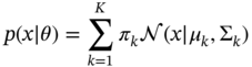
where ![]() are the mixture of weights, such that
are the mixture of weights, such that ![]() . In addition,
. In addition, ![]() denotes the collection of parameters of the model
denotes the collection of parameters of the model ![]() .
.
Now, consider the dataset ![]() , extracted similarly as in Eq. 3.2, and it is assumed that
, extracted similarly as in Eq. 3.2, and it is assumed that ![]() are drawn independent and identically distributed (i.i.d.) from an unknown distribution
are drawn independent and identically distributed (i.i.d.) from an unknown distribution ![]() . The objective here is to find a good approximation of
. The objective here is to find a good approximation of ![]() by means of a GMM with
by means of a GMM with ![]() mixture components and for that the maximum likelihood estimate (MLE) of the parameters
mixture components and for that the maximum likelihood estimate (MLE) of the parameters ![]() need to be obtained [100,101]. The i.i.d. assumption allows the
need to be obtained [100,101]. The i.i.d. assumption allows the ![]() to be written [99,100] as follows:
to be written [99,100] as follows:
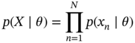
where the individual likelihood term ![]() is a Gaussian mixture density as in Eq. 3.3. Then, it is required to get the log‐likelihood [99,100]
is a Gaussian mixture density as in Eq. 3.3. Then, it is required to get the log‐likelihood [99,100]
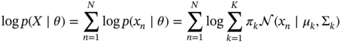
Therefore, the MLE of the model parameters ![]() that maximize the log‐likelihood defined in Eq. 3.5 need to be obtained. The maximum likelihood of the parameters
that maximize the log‐likelihood defined in Eq. 3.5 need to be obtained. The maximum likelihood of the parameters ![]() is estimated using the EM algorithm, which is a general iterative scheme for learning parameters in mixture models.
is estimated using the EM algorithm, which is a general iterative scheme for learning parameters in mixture models.
GMM is one of the most popular classification techniques among SER researchers, and many research works are based on GMM [12,15,39,52–59]. Although average accuracy achieved not up to the mark, around an average of 74.83–81.94%, but least training time of GMM among the prominent classifiers made it an attractive choice as SER classifier.
GMMs are efficient in modeling multimodal distributions [101] with much have been data points compared to HMMs. Therefore, when global features are extracted from speech for SER, fewer data points are available, but GMMs work better in those scenarios [8]. Moreover, the average training time is minimal for GMM [8].
3.4.2.1 Difficulties in Using GMM for SER
Following difficulties in using GMM have been identified:
3.4.3 Support Vector Machine
SVM is fundamentally a two‐class or binary classifier. The SVM provides state‐of‐the‐art results in many applications [104]. Possible values for the label or output are usually assumed to be ![]() so that the predictor becomes
so that the predictor becomes ![]() , where
, where ![]() is the predictor and
is the predictor and ![]() is the dimension of the feature vector. Therefore, given the training dataset of
is the dimension of the feature vector. Therefore, given the training dataset of ![]() data points
data points ![]() , where
, where ![]() and
and ![]() and
and ![]() , the problem is to find the
, the problem is to find the ![]() with least classification error. Consider a linear model of the form
with least classification error. Consider a linear model of the form
to solve this binary classification problem, where ![]() is the weight vector and
is the weight vector and ![]() is the bias. Also, assume that the dataset is linearly separable in the feature space and the objective here is to find the separating hyperplane that maximizes the margin between the positive and negative examples, which means
is the bias. Also, assume that the dataset is linearly separable in the feature space and the objective here is to find the separating hyperplane that maximizes the margin between the positive and negative examples, which means ![]() when
when ![]() and
and ![]() when
when ![]() . Now, the requirement that the positive and the negative examples nearest to the hyperplane to be at least one unit away from the hyperplane yields the condition
. Now, the requirement that the positive and the negative examples nearest to the hyperplane to be at least one unit away from the hyperplane yields the condition ![]() [100]. This condition is known as the canonical representation of the decision hyperplane. Here, the optimization problem is to maximize the distance to the margin, defined in terms of
[100]. This condition is known as the canonical representation of the decision hyperplane. Here, the optimization problem is to maximize the distance to the margin, defined in terms of ![]() as
as ![]() , which is equivalent to minimizing
, which is equivalent to minimizing ![]() , that is
, that is

Equation 3.7 is known as the hard margin, which is an example of quadratic programming. The margin is called hard because the formulation does not allow any violation of margin condition.
The assumption of a linearly separable dataset needs to be relaxed for better generalization of the data because, in practice, the class conditional distributions may overlap. This is achieved by the introduction of a slack variable ![]() where
where ![]() , with each training data point [105,106], which updates the optimization problem as follows
, with each training data point [105,106], which updates the optimization problem as follows
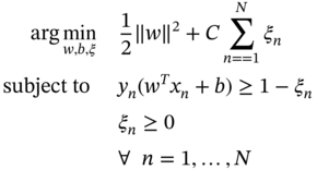
where ![]() manages the size of the margin and the total amount of slack that we have. This model allows some data points to be on the wrong side of the hyperplane to reduce the impact of overfitting.
manages the size of the margin and the total amount of slack that we have. This model allows some data points to be on the wrong side of the hyperplane to reduce the impact of overfitting.
Various methods have been proposed to combine multiple two‐class SVMs to build a multiclass classifier. One of the commonly used approaches is the one‐versus‐the‐rest approach [107], where ![]() separate SVMs are constructed where
separate SVMs are constructed where ![]() is the number of classes and
is the number of classes and ![]() . The
. The ![]() th model
th model ![]() is trained using the data from class
is trained using the data from class ![]() as the positive examples and the data from the remaining
as the positive examples and the data from the remaining ![]() classes as negative examples. There is another approach called one‐versus‐one, where all possible pairs of classes are trained in
classes as negative examples. There is another approach called one‐versus‐one, where all possible pairs of classes are trained in ![]() different two‐class SVM classifiers. Platt [108] proposed the directed acyclic graph support vector machine (DAGSVM), directed acyclic graph SVM.
different two‐class SVM classifiers. Platt [108] proposed the directed acyclic graph support vector machine (DAGSVM), directed acyclic graph SVM.
SVM is extensively used in SER [48,49,55,65–71]. Performance of SVM for SER task in most of the research studies carried out yielded nearly close results, and accuracy is varying around 80% mark. However, Hassan and Damper [69] achieved 92.3% and 94.6% classification accuracy using linear and hierarchical kernels, respectively. They have used a linear kernel instead of a nonlinear radial basis function (RBF) kernel because of very high dimensional features space [72]. Hu et al. [73] explored GMM supervector‐based SVM with different kernels like linear, RBF, polynomial, and GMM KL divergence and found that GMM KL performed the best in classifying emotions.
3.4.3.1 Difficulties with SVM
There is no systematic way to choose the kernel functions, and hence, the separability of transformed features is not guaranteed. Moreover, in SER, complete separation in training data is not recommended to avoid overfitting.
3.4.4 Deep Learning
Deep feedforward networks or multilayer perceptrons (MLPs) are the pure forms of DL models. The objective of an MLP is to approximate some function ![]() such that a classifier,
such that a classifier, ![]() , maps an input
, maps an input ![]() to a category
to a category ![]() . An MLP defines a mapping
. An MLP defines a mapping ![]() , where
, where ![]() is a set of parameters and learns the value of the parameters
is a set of parameters and learns the value of the parameters ![]() that result in the best function approximation. Deep networks are represented as a composition of different functions, and a directed acyclic graph describes how those functions are composed together. For example, there might be three functions
that result in the best function approximation. Deep networks are represented as a composition of different functions, and a directed acyclic graph describes how those functions are composed together. For example, there might be three functions ![]() ,
, ![]() , and
, and ![]() connected in a chain to form
connected in a chain to form ![]() , where
, where ![]() is the first layer of the network,
is the first layer of the network, ![]() is the second layer, and so on. The length of the chain gives the depth of the model, and this depth is behind the name deep learning. The last layer of the network is the output layer.
is the second layer, and so on. The length of the chain gives the depth of the model, and this depth is behind the name deep learning. The last layer of the network is the output layer.
The training phase of neural network ![]() is altered to approximate
is altered to approximate ![]() . Each training example
. Each training example ![]() has a corresponding label
has a corresponding label ![]() , and training decides the values for
, and training decides the values for ![]() such that the output layer can produce values close to
such that the output layer can produce values close to ![]() say
say ![]() . However, the behavior of the hidden layers are not directly specified by training data, and that is why those layers are called hidden. The hidden layers bring the nonlinearity into the system by transforming the input
. However, the behavior of the hidden layers are not directly specified by training data, and that is why those layers are called hidden. The hidden layers bring the nonlinearity into the system by transforming the input ![]() , where
, where ![]() is a nonlinear transform. The whole transformation process is done in the hidden layers, which provide a new representation of
is a nonlinear transform. The whole transformation process is done in the hidden layers, which provide a new representation of ![]() . Therefore, now, it is required to learn
. Therefore, now, it is required to learn ![]() and the model is now becomes
and the model is now becomes ![]() , where
, where ![]() is used to learn
is used to learn ![]() and parameters
and parameters ![]() maps
maps ![]() to the desired output. The
to the desired output. The ![]() is the so‐called activation function of the hidden layers of the feedforward network [109].
is the so‐called activation function of the hidden layers of the feedforward network [109].
Most modern neural networks are trained using the MLE, which means the cost function ![]() is the negative log‐likelihood or the cross‐entropy function between the training data and the model distribution. Therefore, the cost function becomes [109]
is the negative log‐likelihood or the cross‐entropy function between the training data and the model distribution. Therefore, the cost function becomes [109]
where ![]() is the model distribution that varies depending on the selected model, and
is the model distribution that varies depending on the selected model, and ![]() is the target distribution from data. The output distribution determines the choice of the output unit. For example, Gaussian output distribution requires a linear output unit, Bernoulli output distribution requires a Sigmoid function, Softmax Units for Multinoulli Output Distributions, and so on. However, the choice of a hidden unit is still an active area of research, but rectified linear units (ReLU) are the most versatile ones that work well in most of the scenarios. Logistic sigmoid and hyperbolic tangent are other two options out of many other functions researchers are using.
is the target distribution from data. The output distribution determines the choice of the output unit. For example, Gaussian output distribution requires a linear output unit, Bernoulli output distribution requires a Sigmoid function, Softmax Units for Multinoulli Output Distributions, and so on. However, the choice of a hidden unit is still an active area of research, but rectified linear units (ReLU) are the most versatile ones that work well in most of the scenarios. Logistic sigmoid and hyperbolic tangent are other two options out of many other functions researchers are using.
Therefore, in the forward propagation, ![]() is produced and the cost function
is produced and the cost function ![]() is computed. Now, the information generated in the form of
is computed. Now, the information generated in the form of ![]() is appropriately processed so that
is appropriately processed so that ![]() parameters can be appropriately chosen. This task is accomplished in two phases, first computing the gradients using the famous back‐propagation algorithm, and in the second phase, the
parameters can be appropriately chosen. This task is accomplished in two phases, first computing the gradients using the famous back‐propagation algorithm, and in the second phase, the ![]() values are updated based on the gradients computed by the backprop algorithm. The
values are updated based on the gradients computed by the backprop algorithm. The ![]() values are updated through methods such as stochastic gradient descent (SGD). The backprop algorithm applies the chain rule recursively to compute the derivatives of the cost function
values are updated through methods such as stochastic gradient descent (SGD). The backprop algorithm applies the chain rule recursively to compute the derivatives of the cost function ![]() .
.
Different variants of DL exist now, but convolutional neural networks (CNNs) [110,111] and recurrent neural networks (RNNs) [112] are the most successful ones. Convolutional networks are neural networks that use convolution in place of general matrix multiplication in at least one of their layers, whereas when feedforward neural networks are extended to include feedback connections, they are called RNNs. RNNs are specialized in processing sequential data.
SER researchers have used CNNs [35,37,83–87], RNNs [36,84,88], or a combination of the two extensively for SER. Shallow one‐layer or two‐layer CNN structures may not be able to learn effectively the affective features that are discriminative enough to distinguish the subjective emotions [85]. Therefore, researchers are recommending a deep structure. Researchers [36,37,89,90] have studied the effectiveness of attention mechanism.
Researchers are applying end‐to‐end DL systems in SER [8491–94], and most of them use arousal‐valence model of emotions. Although using end‐to‐end DL, the average classification accuracy for arousal is 78.16%, which is decent, for valence, and it is pretty low 43.06%. Among other DNN techniques, very recently, a maximum accuracy of 87.32% is achieved by using a fine‐tuned Alex‐Net on Emo‐DB [85]. Han et al. [113] used extreme learning machine (ELM) for classification, where a DNN takes as input the popular acoustic features within a speech segment and produces segment‐level emotion state probability distributions, from which utterance‐level features are constructed.
3.4.4.1 Drawbacks of Using Deep Learning for SER
Although researchers are using the DL architectures extensively for solving the SER problem, DL methods pose the following difficulties:
- Implementation of tensor operations is a complicated task, which results in limited resources [109]. There are limited sets of libraries, such as TensorFlow (https://github.com/tensorflow/tensorflow), Theano (https://github.com/Theano/Theano), PyTorch (https://github.com/pytorch/pytorch), MXNet (https://github.com/apache/incubator-mxnet), and CNTK (https://github.com/Microsoft/CNTK), which provide the service.
- Back‐propagation often involves the summation of many tensors together, which makes the memory management task difficult and often requires substantial computational resources.
- The introduction of DL methods also increased the feature set dimension for SER manifolds, for example, Wöllmer et al. [88] extracted a total 4843 features.
- One crucial question raised by Lorenzo‐Trueba et al. [114] is that how emotional information should be represented as labels for supervised DNN training, e.g. should emotional class and emotional strength be factorized into separate inputs or not?
3.5 Difficulties in SER Studies
SER mystery is not yet solved, and it has been proved to be difficult. Here are the prominent difficulties faced by the researchers.
- The topic called emotion is inherently uncertain. Because the very experience of emotion is very subjective, its expression varies largely from person to person. Moreover, there is little consensus over the definition of emotion. These are the major hurdles to proceed with the research [115]. For example, several studies [51–53,116–119] reported that there is confusion between anger and happiness emotional expression.
- SER is challenging because of the affective gap between the subjective emotions and low‐level features [85]. Also, the feature analysis in SER is less studied [113], and researchers are still actively looking for the best feature set.
- Speaker and language dependency of classification results are a concern for building more generic SER systems [120]. The same model gives very different classification results with different datasets. Studies reported [53,81,117,121] the speaker dependency phenomenon and tried to address that issue.
- Standard speech databases are not available for SER research so that new models can be effectively benchmarked. Moreover, the absence of good‐quality natural speech emotional databases is hindering the real‐life implementation of SER systems.
- Cross‐corpora recognition results are low [38,65,122]. This indicates that existing models are not generalizing enough for real‐life implementation.
- Classification between high‐arousal and low‐arousal emotions is achieved more accurately, but for other cases, it is low, which needs to be addressed. Moreover, the accuracy of
 ‐way classification with all the emotions in the database is still very low.
3.6 Conclusion
This chapter reviewed different phases of SER. The primary focus is on four prominent classification techniques used in SER to date. HMM was the first technique that has seen some success and then GMM and SVM propelled that progress forward. Also, presently DL techniques, mainly CNN–long short‐term memory (LSTM) combination, is providing state of the art classification performance. However, things have not changed much in case of selecting a feature set for SER because low‐level descriptors (LLD) are still one of the prominent choices, although some researchers in recent times are trying DL techniques for feature learning. The nature of SER databases are changing, and features such as facial expressions and body movements are being included along with the spoken utterances. However, the availability of quality databases is still a challenge.
This work is a survey of current research work in the SER system. Specifically, the classification models used in SER are discussed in more detail, while the features and databases are briefly mentioned. A long list of articles have been referred to during this study, and eight classification models have been identified, which are being used by researchers. However, four classification models have been identified as more effective for SER than the rest. Those four classification models are HMM, GMM, SVM, and DL, which are discussed in the context of SER with a relevant mathematical background. Their drawbacks are also highlighted.
Research results show that DL models are performing significantly better than HMM, GMM, and SVM. The classification accuracy for SER has improved with the introduction of DL techniques because of their higher capacity to learn the underlying pattern in the emotional speech signal. The DL architectures are evolving each day with more and more improvement in classification accuracy of SER speech signals. It is observed that the SER field is still facing many challenges, which are barring research outputs from being implemented as an industry‐grade product. It is also noticed during this study that research work related to feature set enhancement is much less compared to the works done on enhancing classification techniques. However, the available classification techniques in ML field are in a very advanced state, and with the right feature set, they can yield very high classification accuracy rates. DL as a sub‐field of ML, even achieved state‐of‐the‐art classification accuracy in many fields like computer vision, text mining, automatic speech recognition, to name a few. Therefore, the classification technique should not be a hindrance for SER anymore; only the appropriate feature set needs to be fed into the classification system.
References
- 1 Darwin, C. (1948). The Expression of Emotion in Man and Animals. Watts and Co.
- 2 Fairbanks, G. and Pronovost, W. (1938). Vocal pitch during simulated emotion. Science 88 (2286): 382–383. https://doi.org/10.1126/science.88.2286.382.
- 3 Freedman, D.G., Loring, C.B., and Martin, R.M. (1967). Emotional behavior and personality development. In: Infancy and Early Childhood. (ed. Y. Brackbill), 429–502. New York: Free Press.
- 4 Williams, C.E. and Stevens, K.N. (1969). On determining the emotional state of pilots during flight: an exploratory study. Aerospace Medicine 40: 1369–1372.
- 5 Williams, C.E. and Stevens, K.N. (1972). Emotions and speech: some acoustical correlates. The Journal of the Acoustical Society of America 52 (4B): 1238–1250. https://doi.org/10.1121/1.1913238.
- 6 Williamson, J. (1978). Speech analyzer for analyzing pitch or frequency perturbations in individual speech pattern to determine the emotional state of the person. https://patents.google.com/patent/US4093821.
- 7 Picard, R.W. (1997). Affective Computing. Cambridge, MA: MIT Press.ISBN: 0‐262‐16170‐2.
- 8 El Ayadi, M., Kamel, M.S., and Karray, F. (2011). Survey on speech emotion recognition: features, classification schemes, and databases. Pattern Recognition 44 (3): 572–587.
- 9 Sreenivasa Rao, K. and Koolagudi, S.G. (2013). Emotion Recognition using Speech Features. New York: Springer‐Verlag.
- 10 Gnjatovic, M. and Rosner, D. (2010). Inducing genuine emotions in simulated speech‐based human‐machine interaction: the nimitek corpus. IEEE Transactions on Affective Computing 1 (2): 132–144. https://doi.org/10.1109/T-AFFC.2010.14.
- 11 Ververidis, D. and Kotropoulos, C. (2006). Emotional speech recognition: resources, features, and methods. Speech Communication 48 (9): 1162–1181. https://doi.org/10.1016/j.specom.2006.04.003.
- 12 Breazeal, C. and Aryananda, L. (2002). Recognition of affective communicative intent in robot‐directed speech. Autonomous Robots 12 (1): 83–104. https://doi.org/10.1023/A:1013215010749.
- 13 Campbell, N. (2000). Databases of emotional speech.
- 14 Engberg, I.S., Hansen, A.V., Andersen, O., and Dalsgaard, P. (1997). Design, recording and verification of a Danish emotional speech database. In: Proceedings of the 5th European Conference on Speech Communication and Technology.
- 15 Slaney, M. and McRoberts, G. (2003). Babyears: a recognition system for affective vocalizations. Speech Communication 39: 367–384.
- 16 Lee, C.M. and Narayanan, S. (2005). Toward detecting emotions in spoken dialogs. IEEE Transactions on Speech and Audio Processing 13: 293–303.
- 17 Ververidis, D. and Kotropoulos, C. (2003). A state of the art review on emotional speech databases. In: Proceedings of the 1st Richmedia Conference, 109–119. https://www.researchgate.net/publication/50342391_A_State_of_the_Art_Review_on_Emotional_Speech_Databases
- 18 Cowie, R. and Cornelius, R.R. (2003). Describing the emotional states that are expressed in speech. Speech Communication 40 (1): 5–32. https://doi.org/10.1016/S0167-6393(02)00071-7.
- 19 Bänziger, T. and Scherer, K.R. (2005). The role of intonation in emotional expressions. Speech Communication 46 (3): 252–267. https://doi.org/10.1016/j.specom.2005.02.016. Quantitative Prosody Modelling for Natural Speech Description and Generation.
- 20 Rao, K.S. and Yegnanarayana, B. (2006). Prosody modification using instants of significant excitation. IEEE Transactions on Audio, Speech, and Language Processing 14 (3): 972–980. https://doi.org/10.1109/TSA.2005.858051.
- 21 Cowie, R., Douglas‐Cowie, E., Tsapatsoulis, N et al. (2001). Emotion recognition in human‐computer interaction. IEEE Signal Processing Magazine 18 (1): 32–80. https://doi.org/10.1109/79.911197.
- 22 Murray, I. and Arnott, J. (1993). Toward the simulation of emotion in synthetic speech: a review of the literature on human vocal emotion. The Journal of the Acoustical Society of America 93: 1097–1108. https://doi.org/10.1121/1.405558.
- 23 Cowie, R. and Douglas‐Cowie, E. (1996). Automatic statistical analysis of the signal and prosodic signs of emotion in speech 3 (11): 1989–1992. https://doi.org/10.1109/ICSLP.1996.608027.
- 24 Banse, R. and Scherer, K. (1996). Acoustic profiles in vocal emotion expression. Journal of Personality and Social Psychology 70: 614–636. https://doi.org/10.1037/0022-3514.70.3.614.
- 25 Oster, A. and Risberg, A. (1986). The identification of the mood of a speaker by hearing impaired listeners. Speech Transmission Laboratory. Quarterly Progress and Status Reports 27: 79–90.
- 26 Beeke, S., Wilkinson, R., and Maxim, J (2009). Prosody as a compensatory strategy in the conversations of people with agrammatism. Clinical Linguistics & Phonetics 23: 133–155. https://doi.org/10.1080/02699200802602985.
- 27 Borchert, M. and Dusterhoft, A. (2005). Emotions in speech ‐ experiments with prosody and quality features in speech for use in categorical and dimensional emotion recognition environments. In: 2005 International Conference on Natural Language Processing and Knowledge Engineering, 147–151.ISBN: 0‐7803‐9361‐9. https://doi.org/10.1109/NLPKE.2005.1598724.
- 28 Tao, J., Kang, Y., and Li, A. (2006). Prosody conversion from neutral speech to emotional speech. IEEE Transactions on Audio, Speech, and Language Processing 14 (4): 1145–1154. https://doi.org/10.1109/TASL.2006.876113.
- 29 Scherer, K (1986). Vocal affect expression: a review and a model for future research. Psychological Bulletin 99: 143–165. https://doi.org/10.1037//0033-2909.99.2.143.
- 30 Davitz, J.R. and Beldoch, M. (1964). The Communication of Emotional Meaning, McGraw‐Hill Series in Psychology. Greenwood Press.ISBN: 9780837185279; https://books.google.co.za/books?id=1ggRAQAAIAAJ.
- 31 Rabiner, L.R. and Schafer, R.W. (1978). Digital Processing of Speech Signals, Prentice‐Hall Signal Processing Series. Prentice‐Hall.ISBN: 9780132136037. https://books.google.co.za/books?id=YVtTAAAAMAAJ.
- 32 Hernando, J. and Nadeu, C. (1997). Linear prediction of the one‐sided autocorrelation sequence for noisy speech recognition. IEEE Transactions on Speech and Audio Processing 5 (1): 80–84. https://doi.org/10.1109/89.554273.
- 33 Le Bouquin, R. (1996). Enhancement of noisy speech signals: application to mobile radio communications. Speech Communication 18 (1): 3–19. https://doi.org/https://doi.org/10.1016/0167-6393(95)00021-6.
- 34 Bou‐Ghazale, S.E., and Hansen, J.H.L. (2000). A comparative study of traditional and newly proposed features for recognition of speech under stress. IEEE Transactions on Speech and Audio Processing 8 (4): 429–442. https://doi.org/10.1109/89.848224.
- 35 Chen, M., He, X., Yang, J., and Zhang, H. (2018). 3‐D convolutional recurrent neural networks with attention model for speech emotion recognition. IEEE Signal Processing Letters 25 (10): 1440–1444. https://doi.org/10.1109/LSP.2018.2860246.
- 36 Mirsamadi, S., Barsoum, E., and Zhang, C. (2017). Automatic speech emotion recognition using recurrent neural networks with local attention. In: 2017 IEEE International Conference on Acoustics, Speech and Signal Processing (ICASSP), 2227–2231. https://doi.org/10.1109/ICASSP.2017.7952552.
- 37 Neumann, M. and N.T. Vu (2017). Attentive convolutional neural network based speech emotion recognition: a study on the impact of input features, signal length, and acted speech. CoRR, abs/1706.00612. http://arxiv.org/abs/1706.00612.
- 38 Schuller, B., Vlasenko, B., Eyben, F. et al. (2010). Cross‐corpus acoustic emotion recognition: variances and strategies. IEEE Transactions on Affective Computing 1 (2): 119–131. https://doi.org/10.1109/T-AFFC.2010.8.
- 39 Mubarak, O.M., Ambikairajah, E., and Epps, J. (2005). Analysis of an MFCC‐based audio indexing system for efficient coding of multimedia sources. In: Proceedings of the 8th International Symposium on Signal Processing and Its Applications, 2005, vol. 2, 619–622. https://doi.org/10.1109/ISSPA.2005.1581014.
- 40 Roy, T., Marwala, T., and Chakraverty, S. (2018). Precise detection of speech endpoints dynamically: a wavelet convolution based approach. Communications in Nonlinear Science and Numerical Simulation. https://doi.org/https://doi.org/10.1016/j.cnsns.2018.07.008.
- 41 Clore, G.L. and Huntsinger, J.R. (2007). How emotions inform judgment and regulate thought. Trends in Cognitive Sciences 11 (9): 393–399.
- 42 Bitouk, D., Verma, R., and Nenkova, A. (2010). Class‐level spectral features for emotion recognition. Speech Communication 52: 613–625.
- 43 Fernandez, R. and Picard, R.W. (2003). Modeling drivers' speech under stress. Speech Communication 40: 145–159.
- 44 Zhou, G., Hansen, J.H.L., and Kaiser, J.F. (2001). Nonlinear feature based classification of speech under stress. IEEE Transactions on Speech and Audio Processing 9: 201–216.
- 45 Nwe, T.L., Foo, S.W., and De Silva, L.C. (2003). Speech emotion recognition using hidden Markov models. Speech Communication 41: 603–623.
- 46 Kamaruddin, N. and Wahab, A. (2009). Features extraction for speech emotion. Journal of Computational Methods in Science and Engineering 9 (1, 2S1): S1–S12. http://dl.acm.org/citation.cfm?id=1608790.1608791.
- 47 Schuller, B., Rigoll, G., and Lang, M. (2003). Hidden Markov model‐based speech emotion recognition. In: 2003 International Conference on Multimedia and Expo. ICME '03. Proceedings (Cat. No.03TH8698), vol. 1, 401–404. https://doi.org/10.1109/ICME.2003.1220939.
- 48 Kwon, O.‐W., Chan, K., Hao, J., and Lee, T.‐W. (2003). Eighth European Conference on Speech Communication and Technology.
- 49 Lee, C.M., Yildirim, S., Bulut, M. et al. (2004). Emotion recognition based on phoneme classes. In: Proceedings of ICSLP, 889–892.
- 50 Philippou‐Hübner, D., Vlasenko, B., Grosser, T., and Wendemuth, A. (2010). Determining optimal features for emotion recognition from speech by applying an evolutionary algorithm. In: INTERSPEECH, 2358–2361.
- 51 Lin, J., Wei, W., Wu, C., and Wang, H. (2014). Emotion recognition of conversational affective speech using temporal course modeling‐based error weighted cross‐correlation model. In: Signal and Information Processing Association Annual Summit and Conference (APSIPA), 2014 Asia‐Pacific, 1–7. https://doi.org/10.1109/APSIPA.2014.7041621.
- 52 Jeon, J.H., Xia, R., and Liu, Y. (2011). Sentence level emotion recognition based on decisions from subsentence segments. In: 2011 IEEE International Conference on Acoustics, Speech and Signal Processing (ICASSP), 4940–4943. https://doi.org/10.1109/ICASSP.2011.5947464.
- 53 Lugger, M. and Yang, B. (2007). The relevance of voice quality features in speaker independent emotion recognition. In: 2007 IEEE International Conference on Acoustics, Speech and Signal Processing ‐ ICASSP '07, vol. 4, IV–17–IV–20. https://doi.org/10.1109/ICASSP.2007.367152.
- 54 Atassi, H. and Esposito, A. (2008). A speaker independent approach to the classification of emotional vocal expressions. In: 2008 20th IEEE International Conference on Tools with Artificial Intelligence, vol. 2, 147–152. https://doi.org/10.1109/ICTAI.2008.158.
- 55 Schuller, B., Rigoll, G., and Lang, M. (2004). Speech emotion recognition combining acoustic features and linguistic information in a hybrid support vector machine‐belief network architecture. In: Proceedings of IEEE ICASSP, vol. 1, I–577–80. https://doi.org/10.1109/ICASSP.2004.1326051.
- 56 Neiberg, D., Elenius, K., and Laskowski, K. (2006). Emotion recognition in spontaneous speech using GMMs. Proceedings of INTERSPEECH.
- 57 Wang, Y. and Guan, L. (2004). An investigation of speech‐based human emotion recognition. In: IEEE 6th Workshop on Multimedia Signal Processing, 2004., 15–18.
- 58 Zhou, Y., Sun, Y., Zhang, J., and Yan, Y. (2009). Speech emotion recognition using both spectral and prosodic features. In: 2009 International Conference on Information Engineering and Computer Science, 1–4. https://doi.org/10.1109/ICIECS.2009.5362730.
- 59 Luengo, I., Navas, E., Hernáez, I., and Sánchez, J. (2005). Automatic emotion recognition using prosodic parameters. INTERSPEECH.
- 60 Dellaert, F., Polzin, T., and Waibel, A. (1996). Recognizing emotion in speech. In: Proceedings of the 4th International Conference on Spoken Language, vol. 3, 1970–1973. https://doi.org/10.1109/ICSLP.1996.608022.
- 61 Pao, T.‐L., Chen, Y.‐T., Yeh, J.‐H., and Liao, W.‐Y. (2005). Combining acoustic features for improved emotion recognition in Mandarin speech. In: Affective Computing and Intelligent Interaction (ed. J. Tao, T. Tan, and R.W. Picard), 279–285. Berlin, Heidelberg: Springer‐Verlag.ISBN: 978‐3‐540‐32273‐3.
- 62 Yu, F., Chang, E., Xu, Y.‐Q., and Shum, H. (2001). Emotion detection from speech to enrich multimedia content. In: IEEE Pacific Rim Conference on Multimedia.
- 63 Petrushin, V. (2000). Emotion recognition in speech signal: experimental study, development, and application. In: ICSLP 2000, 222–225.
- 64 Lee, C.M., Narayanan, S., and Pieraccini, R. (2001). Recognition of negative emotions from the speech signal. In: IEEE Workshop on Automatic Speech Recognition and Understanding, 2001. ASRU '01., 240–243. https://doi.org/10.1109/ASRU.2001.1034632.
- 65 Sun, R. and Moore, E. (2012). A preliminary study on cross‐databases emotion recognition using the glottal features in speech. INTERSPEECH.
- 66 Espinosa, H.P., García, C.A.R., and Pineda, L.V. (2010). Features selection for primitives estimation on emotional speech. In: 2010 IEEE International Conference on Acoustics, Speech and Signal Processing, 5138–5141. https://doi.org/10.1109/ICASSP.2010.5495031.
- 67 Wu, S., Falk, T.H., and Chan, W.‐Y. (2011). Automatic speech emotion recognition using modulation spectral features. Speech Communication 53 (5): 768–785. https://doi.org/https://doi.org/10.1016/j.specom.2010.08.013. Perceptual and Statistical Audition.
- 68 Pierre‐Yves, O. (2003). The production and recognition of emotions in speech: features and algorithms. International Journal of Human‐Computer Studies 59 (1): 157–183. https://doi.org/https://doi.org/10.1016/S1071-5819(02)00141-6. Applications of Affective Computing in Human‐Computer Interaction.
- 69 Hassan, A. and Damper, R.I. (2010). Multi‐class and hierarchical svms for emotion recognition. INTERSPEECH.
- 70 Rozgic, V., Ananthakrishnan, S., Saleem, Shirin et al. (2012). Emotion recognition using acoustic and lexical features. INTERSPEECH.
- 71 Yeh, L.‐Y. and Chi, T.‐S. (2010). Spectro‐temporal modulations for robust speech emotion recognition. INTERSPEECH.
- 72 Hsu, C.W., Chang, C.‐C., and Lin, C.‐J. (2003). A practical guide to support vector classification.
- 73 Hu, H., Xu, M., and Wu, W. (2007). GMM supervector based svm with spectral features for speech emotion recognition. In: 2007 IEEE International Conference on Acoustics, Speech and Signal Processing ‐ ICASSP '07, vol. 4, IV–413–IV–416. https://doi.org/10.1109/ICASSP.2007.366937.
- 74 Zhu, A. and Luo, Q. (2007). Study on speech emotion recognition system in e‐learning. In: Human‐Computer Interaction. HCI Intelligent Multimodal Interaction Environments (ed. J.A. Jacko), 544–552, Berlin, Heidelberg: Springer‐Verlag.ISBN: 978‐3‐540‐73110‐8.
- 75 Petrushin, V. (2000). Emotion in speech: recognition and application to call centers. Proceedings of Artificial Neural Networks in Engineering.
- 76 Nakatsu, R., Solomides, A., and Tosa, N. (1999). Emotion recognition and its application to computer agents with spontaneous interactive capabilities. In: Proceedings IEEE International Conference on Multimedia Computing and Systems, vol. 2, 804–808. https://doi.org/10.1109/MMCS.1999.778589.
- 77 Nicholson, J., Takahashi, K., and Nakatsu, R. (1999). Emotion recognition in speech using neural networks. In: ICONIP'99. ANZIIS'99 ANNES'99 ACNN'99. 6th International Conference on Neural Information Processing. Proceedings (Cat. No.99EX378), vol. 2, 495–501. https://doi.org/10.1109/ICONIP.1999.845644.
- 78 Tato, R., Santos, R., Kompe, R., and Pardo, J.M. (2002). Emotional space improves emotion recognition. INTERSPEECH.
- 79 Wang, Y., Du, S., and Zhan, Y. (2008). Adaptive and optimal classification of speech emotion recognition. In: 2008 4th International Conference on Natural Computation, vol. 5, 407–411. https://doi.org/10.1109/ICNC.2008.713.
- 80 Yildirim, S., Bulut, M., Lee, C.M. et al. (2004). An acoustic study of emotions expressed in speech. INTERSPEECH.
- 81 McGilloway, S., Cowie, R., ED, C. et al. (2000). Approaching automatic recognition of emotion from voice: a rough benchmark. Proceedings of the ISCA ITRW on Speech and Emotion.
- 82 Ververidis, D., Kotropoulos, C., and Pitas, I. (2004). Automatic emotional speech classification. In: 2004 IEEE International Conference on Acoustics, Speech, and Signal Processing, vol. 1, I–593. https://doi.org/10.1109/ICASSP.2004.1326055.
- 83 Parthasarathy, S. and Tashev, I. (2018). Convolutional neural network techniques for speech emotion recognition. 2018 16th International Workshop on Acoustic Signal Enhancement (IWAENC).
- 84 Trigeorgis, G., Ringeval, F., Brueckner, R. et al. (2016). Adieu features? End‐to‐end speech emotion recognition using a deep convolutional recurrent network. In: 2016 IEEE International Conference on Acoustics, Speech and Signal Processing (ICASSP), 5200–5204. https://doi.org/10.1109/ICASSP.2016.7472669.
- 85 Zhang, S., Zhang, S., Huang, T., and Gao, W. (2018). Speech emotion recognition using deep convolutional neural network and discriminant temporal pyramid matching. IEEE Transactions on Multimedia 20 (6): 1576–1590. https://doi.org/10.1109/TMM.2017.2766843.
- 86 Mao, Q., Dong, M., Huang, Z., and Zhan, Y. (2014). Learning salient features for speech emotion recognition using convolutional neural networks. IEEE Transactions on Multimedia 16 (8): 2203–2213. https://doi.org/10.1109/TMM.2014.2360798.
- 87 Huang, Z., Dong, M., Mao, Q., and Zhan, Y. (2014). Speech emotion recognition using CNN. In: Proceedings of the 22nd ACM International Conference on Multimedia, MM '14, 801–804. New York, NY, USA: ACM.ISBN: 978‐1‐4503‐3063‐3. https://doi.org/10.1145/2647868.2654984.
- 88 Wöllmer, M., Eyben, F., Reiter, S. et al. (2008). Abandoning emotion classes ‐ towards continuous emotion recognition with modelling of long‐range dependencies. INTERSPEECH.
- 89 Huang, C. and Narayanan, S.S. (2017). Deep convolutional recurrent neural network with attention mechanism for robust speech emotion recognition. In: 2017 IEEE International Conference on Multimedia and Expo (ICME), 583–588. https://doi.org/10.1109/ICME.2017.8019296.
- 90 Huang, C.‐W. and Narayanan, S. (2016). Attention assisted discovery of sub‐utterance structure in speech emotion recognition. INTERSPEECH.
- 91 Tzirakis, P., Zhang, J., and Schuller, B.W. (2018). End‐to‐end speech emotion recognition using deep neural networks. In: 2018 IEEE International Conference on Acoustics, Speech and Signal Processing (ICASSP), 5089–5093. https://doi.org/10.1109/ICASSP.2018.8462677.
- 92 Han, J., Zhang, Z., Ringeval, F., and Schuller, B. (2017). Reconstruction‐error‐based learning for continuous emotion recognition in speech. In: 2017 IEEE International Conference on Acoustics, Speech and Signal Processing (ICASSP), 2367–2371. https://doi.org/10.1109/ICASSP.2017.7952580.
- 93 Han, J., Zhang, Z., Ringeval, F., and Schuller, B. (2017). Prediction‐based learning for continuous emotion recognition in speech. In: 2017 IEEE International Conference on Acoustics, Speech and Signal Processing (ICASSP), 5005–5009. https://doi.org/10.1109/ICASSP.2017.7953109.
- 94 Schmitt, M., Ringeval, F., and Schuller, B.W. (2016). At the border of acoustics and linguistics: bag‐of‐audio‐words for the recognition of emotions in speech. INTERSPEECH.
- 95 Rabiner, L. and Juang, B. (1986). An introduction to hidden Markov models. IEEE ASSP Magazine 3 (1): 4–16. https://doi.org/10.1109/MASSP.1986.1165342.
- 96 Ephraim, Y. and Merhav, N. (2002). Hidden Markov processes. IEEE Transactions on Information Theory 48: 1518–1569. https://doi.org/10.1109/TIT.2002.1003838.
- 97 Stamp, Mark (2017). A revealing introduction to hidden markov models. In: Introduction to Machine Learning with Applications in Information Security, 7–35. Chapman and Hall.ISBN: 9781138626782
- 98 Dempster, A., Laird, N., and Rubin, D.B. (1977). Maximum likelihood from incomplete data via em algorithm. Journal of the Royal Statistical Society, Series B 39: 1–38. https://doi.org/10.1111/j.2517-6161.1977.tb01600.x.
- 99 Bishop, C.M. (2007). Pattern Recognition and Machine Learning. New York: Springer‐Verlag.ISBN: 978‐0‐387‐31073‐2.
- 100 Deisenroth, M.P., Faisal, A.A., and Ong, C.S. (2019). Mathematics for Machine Learning. Cambridge University Press.
- 101 Bishop, Christopher M (2005). Neural Networks for Pattern Recognition, vol. 227. Oxford university press.ISBN: 978‐0‐19‐853864‐6
- 102 El Ayadi, M., Kamel, M.S., and Karray, F. (2007). Speech emotion recognition using gaussian mixture vector autoregressive models. 2007 IEEE International Conference on Acoustics, Speech and Signal Processing ‐ ICASSP '07, vol. 4, IV–957. https://doi.org/10.1109/ICASSP.2007.367230.
- 103 Reynolds, D.A. and Rose, R.C. (1995). Robust text‐independent speaker identification using Gaussian mixture speaker models. IEEE Transactions Speech and Audio Processing 3: 72–83.
- 104 Steinwart, I. and Christmann, A. (2008). Support Vector Machines. Springer.
- 105 Bennett, K. and Mangasarian, O.L. (2002). Robust linear programming discrimination of two linearly inseparable sets. Optimization Methods and Software 1: (01): 23–34. https://doi.org/10.1080/10556789208805504.
- 106 Cortes, C. and Vapnik, V. (1995). Support‐vector networks. Machine Learning 20: 273–297. https://doi.org/10.1007/BF00994018.
- 107 Vapnik, V.N. (1998). Statistical Learning Theory. Wiley.
- 108 Platt, J. (2000). Probabilities for SV machines. In: Advances in Large Margin Classifiers (ed. A.J. Smola, P.L. Bartlett, B. Scholkopf, and D. Shuurmans), 61–73. MIT Press.
- 109 Goodfellow, I., Bengio, Y., and Courville, A. (2016). Deep Learning. MIT Press. http://www.deeplearningbook.org.
- 110 Lecun, Y., Bottou, L., Bengio, Y., and Haffner, P. (1998). Gradient‐based learning applied to document recognition. Proceedings of the IEEE 86 (11): 2278–2324. https://doi.org/10.1109/5.726791.
- 111 LeCun, Y., Boser, B., Denker, J.S. et al. (1989). Backpropagation applied to handwritten zip code recognition. Neural Computation 1 (4): 541–551. https://doi.org/10.1162/neco.1989.1.4.541.
- 112 Rumelhart, D., Hinton, G., and Williams, R. (1986). Learning representations by back‐propagating errors. Nature 323: 533–536.
- 113 Han, K., Yu, D., and Tashev, I. (2014). Speech emotion recognition using deep neural network and extreme learning machine. Proceedings of INTERSPEECH.
- 114 Lorenzo‐Trueba, J., Henter, G.E., Takaki, S. et al. (2018). Investigating different representations for modeling and controlling multiple emotions in DNN‐based speech synthesis. Speech Communication 99: 135–143. https://doi.org/https://doi.org/10.1016/j.specom.2018.03.002.
- 115 Schröder, M. and Cowie, R. (2006). Issues in emotion‐oriented computing – towards a shared understanding. Workshop on Emotion and Computing, HUMAINE.
- 116 Amir, N., Kerret, O., and Karlinski, D. (2001). Classifying emotions in speech: a comparison of methods. INTERSPEECH.
- 117 Grimm, M., Kroschel, K., Mower, E., and Narayanan, S. (2007). Primitives‐based evaluation and estimation of emotions in speech. Speech Communication 49 (10): 787–800. https://doi.org/https://doi.org/10.1016/j.specom.2007.01.010. Intrinsic Speech Variations.
- 118 Kim, J., Lee, S., and Narayanan, S. (2010). An exploratory study of manifolds of emotional speech. In: 2010 IEEE International Conference on Acoustics, Speech and Signal Processing, 5142–5145. https://doi.org/10.1109/ICASSP.2010.5495032.
- 119 Ververidis, D. and Kotropoulos, C. (2005). Emotional speech classification using Gaussian mixture models. In: 2005 IEEE International Symposium on Circuits and Systems, vol. 3, 2871–2874. https://doi.org/10.1109/ISCAS.2005.1465226.
- 120 Koolagudi, S.G. and Rao, K.S. (2010). Real life emotion classification using VOP and pitch based spectral features. In: 2010 Annual IEEE India Conference (INDICON), 1–4. https://doi.org/10.1109/INDCON.2010.5712728.
- 121 Kim, J., Park, J., and Oh, Y. (2011). On‐line speaker adaptation based emotion recognition using incremental emotional information. In: 2011 IEEE International Conference on Acoustics, Speech and Signal Processing (ICASSP), 4948–4951. https://doi.org/10.1109/ICASSP.2011.5947466.
- 122 Shami, M. and Verhelst, W. (2007). An evaluation of the robustness of existing supervised machine learning approaches to the classification of emotions in speech. Speech Communication 49 (3): 201–212. https://doi.org/https://doi.org/10.1016/j.specom.2007.01.006.