5
Multimodal Data Representation and Processing Based on Algebraic System of Aggregates
Yevgeniya Sulema1and Etienne Kerre2
1Department of Computer Systems Software, Faculty of Applied Mathematics, Igor Sikorsky Kyiv Polytechnic Institute, Kyiv, 03056, Ukraine
2Department of Applied Mathematics, Computer Science and Statistics, Ghent University, Ghent, B9000, Belgium
5.1 Introduction
In many cases, we can face with a task of collecting data of different nature obtained (registered, recorded, and measured) in different time slots from sources of different types. For example, long‐life medical observation of a patient is such a case: data about a patient's health status can be obtained from a wide range of medical equipment and tools that can be both digital (e.g. a magnetic imaging system) and nondigital (e.g. a mercury thermometer), as well as these datasets can be registered both in paper notes such as the so‐called “patient's medical card” and by using electronic medical documenting systems. The next task after data collection is data synchronization. This task is a part of a wider task of data analysis of all collected multimodal datasets in order to get a whole picture on the object (subject, process, and event) status, behavior, further states, etc.
One of the possible ways toward solving the task of multimodal data analysis is presenting data sets describing the same object as a complex data structure called an aggregate introduced in the Algebraic System of Aggregates (ASA) [1,2].
Formally, an aggregate A is a tuple of arbitrary tuples, whose elements belong to certain sets [1,2]:
where {A} is a tuple of sets Mj and 〈A〉 is a tuple of element tuples ![]() corresponding to the tuple of sets (
corresponding to the tuple of sets (![]() ).
).
If multimodal data are defined (registered, recorded, and measured) in terms of time, an aggregate must have a time value sequence as the first tuple. Such timewise aggregate is called a multi‐image [1,2]. The multi‐image is a data structure that describes an object in such complete way as it is enabled by the available data. Thus, a multi‐image is a nonempty aggregate formalized as:
where T is a set of time values; τ ≥ ni, i ∈ [1, …, N].
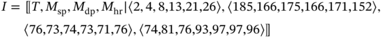
For example, if there are three tuples of the values measured simultaneously, namely, systolic blood pressure (sp), diastolic blood pressure (dp), and heart rate (hr), as well as there is a tuple of time moments when these values are being measured, then we can present all the measurements as one complex data structure – a multi‐image I:
However, the composition of multimodal data in one multi‐image becomes a nontrivial task if the data values have been measured in different time moments. To process such data sequences, we need to synchronize them at first. This task is especially important in cases when multimodal data are being collected for a relatively long time from sources of different types such as remote sensors, paper archives, cloud storages, etc.
In this chapter, we discuss operations on multimodal data and relations between them, which enable complex representation of multiple multimodal data sequences obtained with respect to time in order to compose multi‐images and process them. We pay special attention to multimodal data synchronization by using both crisp and fuzzy approaches.
5.2 Basic Statements of ASA
The ASA is an algebraic system [3–6] that consists of sets (M, F, R), where M is a nonempty set (carrier), whose elements are the elements of the system, F is a set of operations, and R is a set of relations.
As mentioned above, the carrier of ASA is an arbitrary set of specific structures called aggregates. Tuple elements in an aggregate A can have both crisp values ai and fuzzy values ![]() .
.
A tuple element can be empty ∅; a tuple may be empty as well. For example, in Eq. (5.3), the second tuple is empty.
If an aggregate consists of only empty tuples, it is called an empty aggregate: ![]()
An aggregate that does not include any component is called a null‐aggregate: A∅ = 〚∅ ∣ 〈∅〉〛. The null‐aggregate plays a role of a neutral element in ASA.
A tuple element can be undefined, and its notation is _. A tuple may be undefined as well. If an aggregate consists of undefined tuples, it is called an undefined aggregate: ![]() The practical meaning of an undefined aggregate is that we can predefine a data structure (aggregate) even if data sequences are currently unavailable, e.g. if remote sensors are off and, thus, data are not received yet; however, we know their type and can predefine the aggregate sets and tuples.
The practical meaning of an undefined aggregate is that we can predefine a data structure (aggregate) even if data sequences are currently unavailable, e.g. if remote sensors are off and, thus, data are not received yet; however, we know their type and can predefine the aggregate sets and tuples.
The aggregate length ∣ A∣ is the quantity of tuples in it. The length of the empty aggregate ![]() is ∣ A∣ = N. The length of the undefined aggregate
is ∣ A∣ = N. The length of the undefined aggregate ![]() is also ∣ A∣ = N. At the same time, the length of the null‐aggregate is ∣ A∅∣ = 0.
is also ∣ A∣ = N. At the same time, the length of the null‐aggregate is ∣ A∅∣ = 0.
The sequence order of sets and corresponding tuples in an aggregate defines how operations on the aggregate will be fulfilled. In this regard, two aggregates, A1 and A2, can be compatible, A1 ≑ A2, quasi‐compatible, A1 ≐ A2, incompatible, A1 ≗ A2, or hiddenly compatible, A1(≑)A2.
- Aggregates A1 and A2 are compatible if {A1} ≡ {A2}, i.e. both aggregates have the same set of sets and the sequence order of the sets in both aggregates is the same.
- Aggregates A1 and A2 are quasi‐compatible if {A1} ≢ {A2} and {A1} ∩ {A2} ≠ ∅, i.e. the type and sequence order of these aggregates coincide partly.
- Aggregates A1 and A2 are incompatible if {A1} ∩ {A2} = ∅.
- Aggregates A1 and A2 are hiddenly compatible if {A1} ≢ {A2}, ∣ A1∣ = ∣ A2∣ = N, and ∀Mj ⊂ {Ak}, j = [1, … , N], k = [1, 2], i.e. both aggregates have the same set of sets, but the order of these sets differs.
For example, let the sets be defined in the following way:
- Mt = [35.0, …, 39.9] is a set of temperature values (°C);
- Mhr = [50, …, 110] is a set of heart rate values (bpm);
- Msp = [80, …, 190] is a set of systolic pressure values (mmHg);
- Mdp = [55, …, 100] is a set of diastolic pressure values (mmHg).
Let us consider the following aggregates whose elements belong to these sets:
- A1 = 〚Mt, Mhr ∣ 〈36.4,36.1,36.3,36.2,36.5,36.3〉, 〈75,76,74,73,75,75〉〛;
- A2 = 〚Mt, Mhr ∣ 〈36.5,36.5,36.8,36.6,36.3,36.4,37.0,36.5〉, 〈74,81,76,93,97,97,96〉〛;
- A3 = 〚Msp, Mdp ∣ 〈185,166,175,166,171,152〉, 〈76,73,74,73,71,76〉〛;
- A4 = 〚Mt, Msp ∣ 〈36.5,36.5,36.8,36.6,36.3,36.4〉, 〈177,159,174,155,167,150〉〛;
- A5 = 〚Mhr, Mt ∣ 〈74,81,76,93,97〉, 〈36.5,36.5,36.3,36.4,37.0,36.5〉〛.
Then, we can conclude that
- – A1 ≑ A2 because the first tuple in both A1 and A2 belongs to set Mt and the second tuple in both A1 and A2 belongs to set Mhr.
- – A1 ≗ A3 because the first tuple of A1 belongs to set Mt, whereas the first tuple of A3 belongs to Msp, as well as the second tuple of A1 belongs to set Mhr, whereas the second tuple of A3 belongs to Mdp.
- – A1 ≐ A4 because the first tuple of both A1 and A4 belongs to set Mt, but at the same time, the second tuple of A1 belongs to set Mhr, whereas the second tuple of A4 belongs to Msp.
- – A1(≑)A5 because now they are incompatible, but they will become compatible if we change the order of tuples in one of them (e.g. in A5):
 . It can be fulfilled by applying an ordering operation to the elements of this tuple.
5.3 Operations on Aggregates and Multi‐images
Operations on aggregates include arithmetical operations, logical operations, and ordering operations. Arithmetical operations include elementwise addition, scalar addition, elementwise subtraction, scalar subtraction, elementwise multiplication, scalar multiplication, elementwise division, and scalar division. The logical operations on aggregates are union; intersection; difference; symmetric difference; and exclusive intersection [1].
The union of two aggregates A1 and A2 is aggregate B, which includes components of both aggregates and is formed according to the following rule:
- If aggregates A1 and A2 are such as A1 ≑ A2 and


then the elements of i‐tuple of A2 are added at the end of i‐tuple of A1:
(5.4)
- If aggregates A1 and A2 are such as A1 ≗ A2 and


then the tuples of A2 are added at the end of the tuple of tuples of A1 and the corresponding sets of A2 are added at the end of the set sequence of A1:
(5.5)
- If aggregates A1 and A2 are such as A1 ≐ A2 and


then the elements of i‐tuple of A2 are added at the end of i‐tuple of A1 if the elements of these tuples belong to the same set; otherwise, the rule for incompatible aggregates is applied:

The intersection of two aggregates A1 and A2 is aggregate B, which includes only common components of both aggregates and is formed according to the following rule:
- If aggregates A1 and A2 are such as A1 ≑ A2 and


then B includes the elements of both aggregates, which are common for them, in every tuple:
(5.7)
where


It means that if we go through elements of
 from its first element
  to its last element
  and compare each next element
  (1 ≤ li ≤ l, where l is the total number of elements in
  ) with elements of
  , then
  is the first element of
  , which is also present in
  , and
, and  is the last element of
  , which is also present in
  .
.Because we find intersection of
 and
and  , we also look for
  and
and  . To find them, we go through elements of
  from its first element
  to its last element
  and compare each next element
  (1 ≤ rj ≤ r, where r is the total number of elements in
  ) with elements of
  , then
  is the first element of
  , which is also present in
  , and
, and  is the last element of
  , which is also present in
  . Finally, the result of intersection of
  and
and  is the tuple with elements
  .
.For example, if
 and
and  , then
  and
and  . At the same time,
  as well as
  . Finally,
  .
. - If aggregates A1 and A2 are such as A1 ≗ A2, then B = A1 ∩ A2 = 〚∅ ∣ 〈∅〉〛 = A∅.
- If aggregates A1 and A2 are such as A1 ≐ A2 and


then B includes elements of both aggregates, which are common for them, only in tuples of common sets; thus, the number of sets shortens. Only considering the common tuples, we proceed as in the first case:
(5.8)
The difference of two aggregates A1 and A2 is aggregate B, which includes only components present in A1 and absent in A2; it is formed according to the following rule:
- If aggregates A1 and A2 are such as A1 ≑ A2 and


then B includes the elements of A1, which are absent in A2, in every tuple:
(5.9)
where


- If aggregates A1 and A2 are such as A1 ≗ A2, then B = A1A2 = A1.
- If aggregates A1 and A2 are such as A1 ≐ A2 and


then B includes the elements of A1, which are absent in A2, in tuples of common sets and all tuples of sets defined only in A1:
(5.10)
where

The symmetric difference of two aggregates A1 and A2 is aggregate B, which includes both components present in A1 and absent in A2 and components present in A2 and absent in A1; it is formed according to the following rule:
- If aggregates A1 and A2 are such as A1 ≑ A2 and


then B includes the elements of A1, which are absent in A2, and elements of A2, which are absent in A1, in every tuple:
(5.11)
where


- If aggregates A1 and A2 are such as A1 ≗ A2 and


then B is equal to the union of A1 and A2:
(5.12)
- If aggregates A1 and A2 are such as A1 ≐ A2 and


then B includes elements of A1, which are absent in A2, and elements of A2, which are absent in A1, in tuples of common sets, all tuples of sets defined only in A1, and all tuples of sets defined only in A2:
(5.13)
where


The exclusive intersection of two aggregates A1 and A2 is aggregate B, which includes only components of A1 common for both aggregates and is formed according to the following rule:
- If aggregates A1 and A2 are such as A1 ≑ A2 and


then B includes the elements of A1, which are common for both A1 and A2, in every tuple:
(5.14)
where

- If aggregates A1 and A2 are such as A1 ≗ A2, then B = A1 ¬ A2 = 〚∅ ∣ 〈∅〉〛 = A∅.
- If aggregates A1 and A2 are such as A1 ≐ A2 and


then B includes the elements of A1, which are common for both A1 and A2, only in tuples of common sets; thus, the number of sets shortens:
(5.15)
where

The difference between exclusive intersection and intersection is that the result of intersection of two aggregates A1 and A2 is the aggregate that includes common components of both aggregates. At the same time, the result of exclusive intersection is the aggregate that includes components of A1, which are also present in A2, but it does not include any components of A2. For example, if we have two compatible aggregates A1 and A2 such as:
Then, intersection gives us A1 ∩ A2 = 〚Mt, Mhr ∣ 〈36.4,36.3,36.5,36.3,36.5,36.5,36.3,36.4,36.5〉, 〈76,74,74,76〉〛. At the same time, exclusive intersection is resulted in A1 ¬ A2 = 〚Mt, Mhr ∣ 〈36.4,36.3,36.5,36.3〉, 〈76, 74〉〛.
If we have two quasi‐compatible aggregates A1 and A3, where A3 is defined as:
Then, we get a result in a similar way but only for the first tuples because they both belong to the same set Mt:
The logical operations in ASA are noncommutative because the sequence order is important in tuples; this property distinguishes them from the logical operations on sets.
Ordering operations include sets ordering, ascending sorting, descending sorting, singling, extraction, and insertion [2].
The sets ordering operation reorders an aggregate according to a template aggregate. The template aggregate can be arbitrary, undefined, or empty.
Let the aggregate A be defined as:
Besides, let the template aggregate Atem be defined as:
Then, the result of sets ordering operation on the aggregates A and Atem is aggregate B defined as:
The sets ordering operation can also be applied to two arbitrary aggregates A1 and A2, where A2 is used as a template. The practical meaning of such operation is that we can reorder one aggregate (A1) according to another aggregate (A2). Thus, if A1(≑)A2, these aggregates become compatible as a result of sets ordering operation and we can further handle them in the same way, e.g. we can compare the first tuple of A1 with the first tuple of A2 and they will be comparable – which was not possible before reordering because the “old” first tuple of A1 and the first tuple of A2 belonged to different sets.
The result of sets ordering operation depends on the aggregates' compatibility:
- – If A1 ≑ A2, then sets ordering operation is resulted in aggregate B, which is equal to A1:

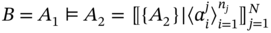
- – If A1 ≐ A2 and there is no hidden compatibility between A1 and A2, then the result of sets ordering operation is empty aggregate:
B = A1 ⊨ A2 = 〚{A2} ∣ 〈∅〉〛.
- – If A1 ≗ A2 and there is no hidden compatibility between A1 and A2, then the result of sets ordering operation is aggregate B:
(5.19)
where
 ,
,  ,
,  , 〈B〉 ≢ 〈A1〉.
 - – If A1(≑)A2, then the result of sets ordering operation is aggregate B such that B ≑ A2 and 〈B〉 ≡ 〈A1〉:
(5.20)
where
 .
.
For example, if we have aggregates A1, A2, and A3 such as A1 ≗ A2, A2(≑) A3, which are defined in the following way:
Then, we can obtain the following results of sets ordering operation:
The sorting operations are ascending sorting and descending sorting. These operations enable reordering of all tuples according to new – sorted – elements order (ascending or descending) of a certain tuple (called a primary tuple) among all tuples of the aggregate.
Let ![]() and ∃k such as 1 < k < N, k ≠ 2 and n1 > nk > nN, n2 = nk. Then, the result of ascending sorting operation of A1 according to the elements of tuple
and ∃k such as 1 < k < N, k ≠ 2 and n1 > nk > nN, n2 = nk. Then, the result of ascending sorting operation of A1 according to the elements of tuple ![]() is aggregate B such as:
is aggregate B such as:

where ![]() and n = nk if nj ≥ nk or n = nj if nj < nk.
and n = nk if nj ≥ nk or n = nj if nj < nk.
The result of descending sorting operation of A1 according to the elements of tuple ![]() is aggregate B such as:
is aggregate B such as:

If k = 1, k = 2, or k = N, the sorting operation is fulfilled by the same principle.
If n1 = n2 = ⋯ = nk = ⋯ = nN, the result of ascending sorting operation is:
and the result of descending sorting operation is:
A variant of the sorting operations is the sorting operations with appending (ascending sorting with appending and descending sorting with appending), which allow to increase the length of shorter tuples according to the length of the primary tuple by adding a value x (x ∈ [∅, _, q], q ∈ Mj, 1 ≤ j ≤ N) either to the end or to the beginning of the shorter tuples.
The result of ascending sorting with appending at the end of the shorter tuples of aggregate A1 is aggregate B:

where ![]() .
.
The result of ascending sorting with appending at the beginning of the shorter tuples of the aggregate A1 is aggregate B:

where ![]() .
.
The result of descending sorting with appending at the end of the shorter tuples of aggregate A1 is aggregate B:

The result of descending sorting with appending at the beginning of the shorter tuples of the aggregate A1 is aggregate B:

If aggregate A1is defined as:

where 1 ≤ k ≤ N, and let ∃ml, ∀ l such as ![]() , then the result of singling operation on aggregate A1 by the tuple
, then the result of singling operation on aggregate A1 by the tuple ![]() is aggregate B such as:
is aggregate B such as:

If there is aggregate A1 defined as:
then the result of extraction operation of the element ![]() from aggregate A1 is aggregate B such as:
from aggregate A1 is aggregate B such as:
The operation of conditional extraction is defined on the assumption of a given condition such as ![]() or
or ![]() . For example:
. For example: ![]() .
.
If there is aggregate A1 defined as:
where 1 ≤ m ≤ N and let ∃d such as ![]() , then the result of insertion operation of d to aggregate A1 can be obtained by using two equivalent ways defined in Eqs. (5.34) and (5.35).
, then the result of insertion operation of d to aggregate A1 can be obtained by using two equivalent ways defined in Eqs. (5.34) and (5.35).


The operation of conditional insertion is defined on the assumption of a given condition such as ![]() or
or ![]() . For example,
. For example, ![]() .
.
The ordering operations in ASA allow us to reorder both elements in tuples and tuples in aggregates (multi‐images).
5.4 Relations and Digital Intervals
Relations in ASA include relations between tuple elements, relations between tuples, and relations between aggregates. Relations between tuple elements are is greater, is less, is equal, proceeds, and succeeds. The first three relations are based on element value and the last two relations concern elements position in a tuple. Naturally, elements must belong to the same tuple. Relations between tuples enable the following types of tuple comparison: arithmetical comparison, frequency comparison, and interval comparison. Arithmetical comparison is elementwise and based on the following relations: is strictly greater, is majority‐vote greater, is strictly less, is majority‐vote less, is strictly equal, and is majority‐vote equal.
Frequency comparison is based on the following relations: is thicker, is rarer, and is equally frequent. Interval comparison is based on the following temporal relations: coincides with, is before, is after, meets, is met by, overlaps, is overlapped by, during, contains, starts, is started by, finishes, and is finished by.
Relations between tuples of aggregates are identical to relations between single tuples defined above: relations of arithmetical comparison, relations of frequency comparison, and relations of interval comparison. However, the possibility of their application depends on the aggregates' compatibility: relations between tuples can be applied only to compatible and quasi‐compatible aggregates. Hiddenly compatible aggregates must be first transformed to compatible ones [2] and then a relation between tuples can be applied to them.
Because a multi‐image, by definition, is an aggregate, all types of relations defined in ASA can be applied to multi‐images as well.
A time tuple in a multi‐image, which is defined by (5.2), can be considered as an interval. However, in contrast with a classical interval, the time tuple consists of a finite number of discrete values. To show the difference between the time tuple and a classical interval, let us first discuss a classical approach of interval‐based temporal logic.
One of the pioneering works related to interval processing is [7], where Allen presented interval algebra and interval‐based temporal logic, including relations between intervals. If X and Y are intervals such as X = [x−, x+] and Y = [y−, y+], the relations between them are defined as shown in Table 5.1.
In [8], Allen and Hayes axiomatized a theory of time in terms of intervals and the single relation meet. They extended Allen's interval‐based theory by formally defining the beginnings and endings of intervals, which have properties normally associated with points. The authors distinguished between these point‐like objects and the concept of a moment as hypothesized in discrete time models.
In these and other related works [9–13], the relations of Allen's interval‐based theory are to be applied to an interval [x−, x+], where x− ≤ x+. However, in ASA, we operate with discrete values and we cannot use Allen's interval‐based theory approaches directly. For example, when we measure data for further composing of a multi‐image, we operate with discrete time values, which being considered all together can be defined as a discrete time interval as it consists of specific discrete time points when the data values have been obtained. Thus, we need to make a transition from an interval [7–13] to a discrete interval.
Let us define a discrete interval as a tuple ![]() , whose elements are unique discrete values
, whose elements are unique discrete values ![]() such as that either ti < ti + 1 or ti > ti + 1 is true for all pairs (ti, ti + 1), ∀i ∈ [1…n − 1], ti ∈ ℝ. Thus, a discrete interval is a strictly increasing or decreasing finite sequence in ℝ.
such as that either ti < ti + 1 or ti > ti + 1 is true for all pairs (ti, ti + 1), ∀i ∈ [1…n − 1], ti ∈ ℝ. Thus, a discrete interval is a strictly increasing or decreasing finite sequence in ℝ.
Then, discrete intervals can be a subject of relations similar to those introduced by Allan in [7]. These temporal relations between two discrete intervals are coincides with, is before, is after, meets, is met by, overlaps, is overlapped by, during, contains, starts, is started by, finishes, and is finished by. Let us define these relations. Note that for consistency with works on Allen's interval algebra, we refer to in this research; hereinafter, we use notion for relations between digital intervals similar to that used in Allen's interval algebra (e.g. ed).
Table 5.1 Allen's interval algebra relations.
| Relation | Notation | Definition |
| X before Y | b(X, Y) | x+ < y− |
| X after Y | bi(X, Y) | x− > y+ |
| X equal Y | e(X, Y) | x− = y− and x+ = y+ |
| X meets Y | m(X, Y) | x+ = y− |
| X is met by Y | mi(X, Y) | x− = y+ |
| X overlaps Y | o(X, Y) | x− < y− and x+ > y−and x+ < y+ |
| X is overlapped by Y | oi(X, Y) | x− > y− and x− < y+ and x+ > y+ |
| X during Y | d(X, Y) | x− > y− and x+ < y− |
| X contains Y | di(X, Y) | x− < y− and x− > y+ |
| X starts Y | s(X, Y) | x− = y− and x+ < y+ |
| X is started by Y | si(X, Y) | x− = y− and x+ > y+ |
| X finishes Y | f(X, Y) | x− > y− and x+ = y+ |
| X is finished by Y | fi(X, Y) | x− < y− and x+ = y+ |
For two discrete intervals ![]() and
and ![]() , we define:
, we define:
- – The relation
 coincides with
  as:
as:
- – The relation
 is before
  as:
as:
- – The relation
 is after
  as:
as:
- – The relation
 meets
meets  as:
as:
- – The relation
 is met by
  as:
as:
- – The relation
 overlaps
  as:
as:
- – The relation
 is overlapped by
  as:
as:
- – The relation
 during
  as:
as:
- – The relation
 contains
  as:
as:
- – The relation
 starts
  as:
as:
- – The relation
 is started by
  as:
as:
- – The relation
 finishes
  as:
(5.47)
as:
(5.47)
- – The relation
 is finished by
  as:
as:
Note that since ![]() and
and ![]() are discrete intervals, there is no requirement that
are discrete intervals, there is no requirement that ![]() and
and ![]() (1 < i < n1, 1 < j < n2) must coincide in such relations as
(1 < i < n1, 1 < j < n2) must coincide in such relations as ![]() ,
, ![]() ,
, ![]() ,
, ![]() ,
, ![]() ,
, ![]() ,
, ![]() ,
, ![]() , and
, and ![]() . For example, if we have two tuples
. For example, if we have two tuples ![]() and
and ![]() as depicted in Figure 5.1.
as depicted in Figure 5.1.
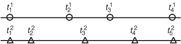
Figure 5.1 An example of two coinciding discrete intervals.
Then, ![]() coincides with
coincides with ![]() because
because ![]() and
and ![]() .
.
In this work, we also introduce the relation between, which can be applied to any number of discrete intervals:
- –
 means that a discrete interval
  is between the discrete values α and β;
 - –
 means that both discrete intervals
  and
and  are between the discrete values α and β;
 - –
 means that all discrete intervals
  ( j ∈ [1…n]) are between the discrete values α and β.
Thus, the relation between for two tuples ![]() and
and ![]() can be defined as follows:
can be defined as follows:
where α and β are given values, α, β ∈ T; T is the time value set.
The relation between for two discrete intervals can be considered as a generalized form of the relation coincides with, because the relation between (5.49) is equivalent to the relation coincides with (5.36) if both ![]() and
and ![]() .
.
5.5 Data Synchronization
Because a multi‐image is a digital representation of a real‐world object (process, phenomenon, event, subject), data tuples of different modalities, which are obtained from different sources (sensors, cloud storages, local storages, computing resources, etc.), need to be synchronized between each other to enable constructing the proper multi‐image as well as to compare and analyze several multi‐images in the same processing procedure. Mathematical models of data synchronization will enable further development of algorithms as well as software for multimodal data processing.
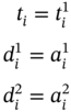
Let us consider two multi‐images I1 and I2, which present a state of the same object of study and are defined as:

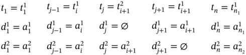
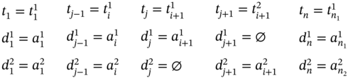
We assume that one characteristic of this object has been measured in time moments ![]() , and as a result, we obtained the data tuple
, and as a result, we obtained the data tuple ![]() ; another characteristic has been measured in time moments
; another characteristic has been measured in time moments ![]() , and as a result, we obtained the data tuple
, and as a result, we obtained the data tuple ![]() . Since I1 and I2 describe different sides of behavior of the same object, our task is to compose a joint multi‐image I that consists of the joint time tuple
. Since I1 and I2 describe different sides of behavior of the same object, our task is to compose a joint multi‐image I that consists of the joint time tuple ![]() and the synchronized data tuples
and the synchronized data tuples ![]() and
and ![]() . The tuple
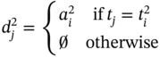
. The tuple ![]() includes values of
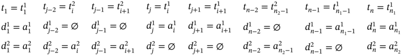
includes values of ![]() and empty elements and is formed according to the rule:
and empty elements and is formed according to the rule:

Similarly, the tuple ![]() includes values of
includes values of ![]() and empty elements and is formed according to the rule:
and empty elements and is formed according to the rule:
In general, the joint multi‐image I is formed as a result of three operations, viz., union defined by (5.6), sorting defined by (5.21), and singling defined by (5.30):
The union enables consolidation of two multi‐images I1 and I2 in one multi‐image ![]() , but if time tuples in I1 and I2, i.e.
, but if time tuples in I1 and I2, i.e. ![]() and
and ![]() , include the same values, then
, include the same values, then ![]() will include duplicated elements and, thus, the synchronization of data tuples
will include duplicated elements and, thus, the synchronization of data tuples ![]() and
and ![]() will be incorrect. To avoid it, we must sort
will be incorrect. To avoid it, we must sort ![]() by time tuple values by using sorting operation and, next, remove duplicated elements in the joint time tuple
by time tuple values by using sorting operation and, next, remove duplicated elements in the joint time tuple ![]() by using singling operation.
by using singling operation.
Let us consider the following practical task as an example. We assume that two parameters, viz., a temperature and an erythrocyte sedimentation rate, have being measured for the same patient during four‐week health status monitoring. Because these measurements are of different nature and fulfilled by different hospital units, we obtain two multi‐images, even if measurements of both types were obtained at the same days of a month:

where
- Mt = [36.0, …, 39.9] is a set of temperature values (°C);
- Mesr = [2, …, 20] is a set of erythrocyte sedimentation rate values (mm/h);
- T = [1, …, 31] is a set of time values (day of a month).
If we try to apply only union operation to I1 and I2, we obtain wrong synchronization because data of different types do not correspond each other: ![]() .
.
To correct it, we need to sort ![]() in ascending order of time values and then remove duplicated time values:
in ascending order of time values and then remove duplicated time values:
Now, all data correspond each other, e.g. we can see that on the 16th day of monitoring, the patient had the body temperature 37.3 °C and the erythrocyte sedimentation rate in his blood test was 15 mm/h.
In this example, we considered the particular case when time values ![]() fully coincide with
fully coincide with ![]() ; however, in a general case, time tuples can be connected with any temporal relation defined by (5.36)–(5.49). Thus, to find time values tj satisfying the condition in (5.51) and/or (5.52), we need to analyze interval relations between time value tuples
; however, in a general case, time tuples can be connected with any temporal relation defined by (5.36)–(5.49). Thus, to find time values tj satisfying the condition in (5.51) and/or (5.52), we need to analyze interval relations between time value tuples ![]() and
and ![]() and compose the joint time value tuple
and compose the joint time value tuple ![]() , which includes all time values from both
, which includes all time values from both ![]() and
and ![]() but do not duplicate them if some of time values in
but do not duplicate them if some of time values in ![]() and
and ![]() coincide. To do this, we need to compare value intervals of
coincide. To do this, we need to compare value intervals of ![]() and
and ![]() .
.
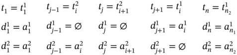
The simplest case is when the measurements of both ![]() and
and ![]() data tuples have been fulfilled simultaneously (hereinafter, we suppose that the data values are obtained from sensors as a result of measuring certain parameters of a physical process; however, the data can also be obtained as a result of modeling, processing, prediction, simulation, etc.). It means that
data tuples have been fulfilled simultaneously (hereinafter, we suppose that the data values are obtained from sensors as a result of measuring certain parameters of a physical process; however, the data can also be obtained as a result of modeling, processing, prediction, simulation, etc.). It means that ![]() and
and ![]() are connected by the relation coincides with. In general, the relation coincides with between two tuples
are connected by the relation coincides with. In general, the relation coincides with between two tuples ![]() and
and ![]() is defined in Eq. (5.36). This relation enables many different subcases depending on a number of values in each data tuple. Let us consider all possible subcases (Figures 5.2–5.4).
is defined in Eq. (5.36). This relation enables many different subcases depending on a number of values in each data tuple. Let us consider all possible subcases (Figures 5.2–5.4).
The first group of subcases for ![]() is when n1 is an even value (n1 mod 2 = 0) and
is when n1 is an even value (n1 mod 2 = 0) and ![]() , i.e.
, i.e. ![]() is equally frequent to
is equally frequent to ![]() ; it means that
; it means that ![]() (i.e. n1 = n2).
(i.e. n1 = n2).
If ![]() , ∀i ∈ [1…n1], then n = n1 and the tuple values of the multi‐image I as introduced in (5.2) are defined in (5.54) and depicted in Figure 5.2a.
, ∀i ∈ [1…n1], then n = n1 and the tuple values of the multi‐image I as introduced in (5.2) are defined in (5.54) and depicted in Figure 5.2a.
The case when ![]() and
and ![]() can be illustrated by Figure 5.2b. Such mutual alignment of the time moments
can be illustrated by Figure 5.2b. Such mutual alignment of the time moments ![]() ,
, ![]() ,
, ![]() , and
, and ![]() , when data values
, when data values ![]() ,
, ![]() ,
, ![]() , and
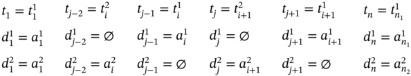
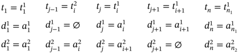
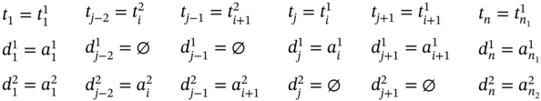
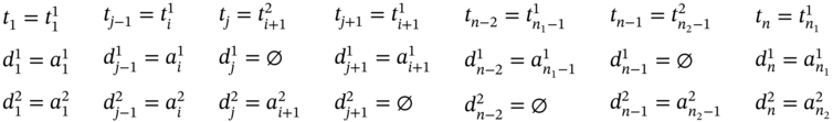
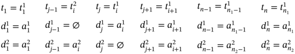
, and ![]() have been measured, requires synchronization of tuple elements which can be stated as:
have been measured, requires synchronization of tuple elements which can be stated as:
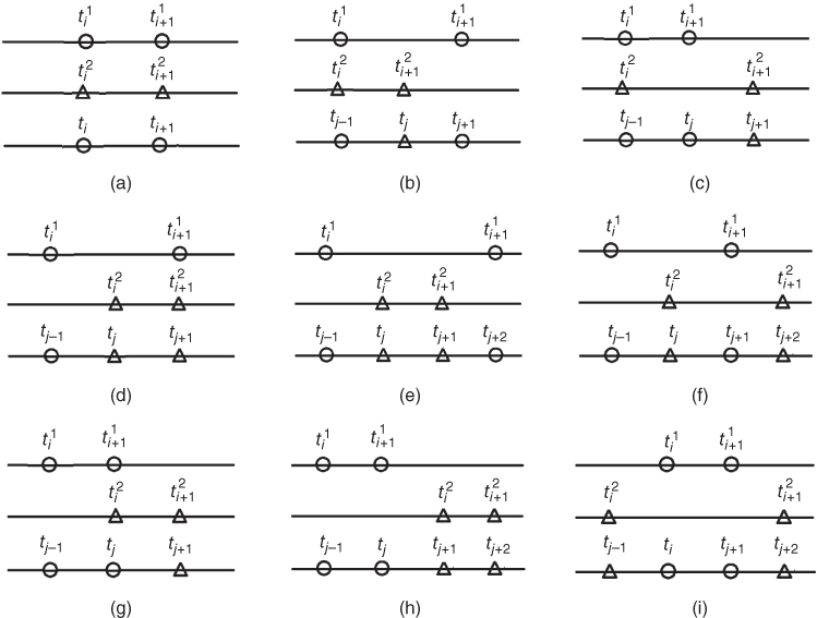

Figure 5.2 The subcases for  when
when  .
.  and
and  are elements of the time tuple
  ;
;  and
and  are elements of the time tuple
  ; tj − 1, tj, tj + 1, and tj + 2 are elements of the synchronized time tuple
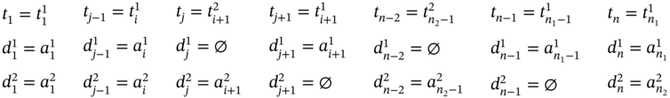
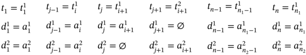
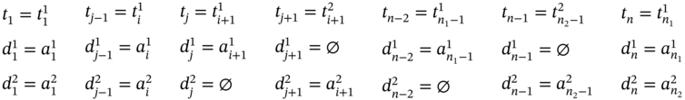
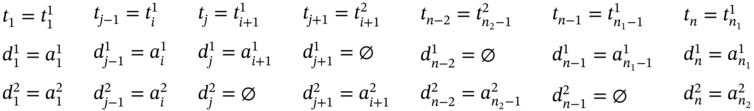
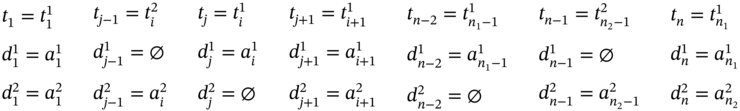
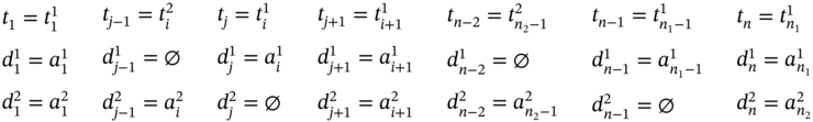
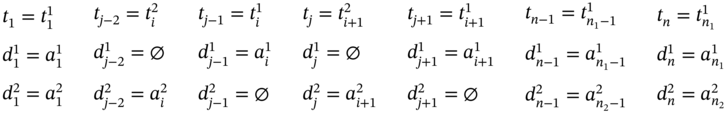
  . For two measurement processes: (a) measurements of both parameters are simultaneous at the current and the next moments of time; (b) the current measurements of both parameters are simultaneous, but the next measurement of the 2nd parameter happens earlier than the next measurement of the 1st parameter; (c) the current measurements of both parameters are simultaneous, but the next measurement of the 1st parameter happens earlier than the next measurement of the 2nd parameter; (d) the current measurement of the 1st parameter happens earlier than the current measurement of the 2nd parameter, but the next measurements of both parameters are simultaneous; (e) the current measurement of the 1st parameter happens earlier than the current measurement of the 2nd parameter, but the next measurement of the 1st parameter happens later than the next measurement of the 2nd parameter; (f) the current and the next measurements of the 1st parameter happen earlier than the current and the next measurements of the 2nd parameter, respectively; (g) the next measurement of the 1st parameter and the current measurement of the 2nd parameter are simultaneous; (h) both measurements of the 1st parameter happen earlier than both measurements of the 2nd parameter; (i) the current measurement of the 1st parameter happens later than the current measurement of the 2nd parameter, but the next measurement of the 1st parameter happens earlier than the next measurement of the 2nd parameter; (j) the current measurement of the 1st parameter happens later than the current measurement of the 2nd parameter, but the next measurements of both parameters are simultaneous; (k) the current and the next measurements of the 1st parameter happen later than the current and the next measurements of the 2nd parameter, respectively; (l) the current measurement of the 1st parameter and the next measurement of the 2nd parameter are simultaneous; (m) both measurements of the 1st parameter happen later than both measurements of the 2nd parameter.

Figure 5.3 The subcases for  when
when  .
.  is an element of the time tuple
  ;
;  and
and  are elements of the time tuple
  ; tj − 1, tj, and tj + 1 are elements of the synchronized time tuple
  . For two measurement processes: (a) the current measurements of both parameters are simultaneous; (b) the current measurement of the 1st parameter happens earlier than the current measurement of the 2nd parameter; (c) the current measurement of the 1st parameter and the next measurement of the 2nd parameter are simultaneous; (d) the current measurement of the 1st parameter happens later than the next measurement of the 2nd parameter; (e) the current measurement of the 1st parameter happens later than the current measurement and earlier than the next measurement of the 2nd parameter.

It means that in time moment ![]() , we have both data values
, we have both data values ![]() and
and ![]() measured (consider the values at the left column above as well as the graphical elements at the left side of Figure 5.2b); in time moment
measured (consider the values at the left column above as well as the graphical elements at the left side of Figure 5.2b); in time moment ![]() , we have only
, we have only ![]() measured (consider the central column as well as the central part of Figure 5.2b); in time moment
measured (consider the central column as well as the central part of Figure 5.2b); in time moment ![]() , we have only
, we have only ![]() measured (consider the right column as well as the right side of Figure 5.2b).
measured (consider the right column as well as the right side of Figure 5.2b).
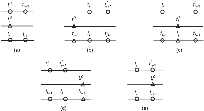
Figure 5.4 The subcases for  when
when  .
.  and
and  are elements of the time tuple
  ;
;  is an element of the time tuple
  ; tj − 1, tj, and tj + 1 are elements of the synchronized time tuple
  . For two measurement processes: (a) the current measurements of both parameters are simultaneous; (b) the current measurement of the 1st parameter happens later than the current measurement of the 2nd parameter; (c) the current measurement of the 2nd parameter happens later than the current measurement and earlier than the next measurement of the 1st parameter; (d) the current measurement of the 2nd parameter happens later than the next measurement of the 1st parameter; (e) the current measurement of the 2nd parameter and the next measurement of the 1st parameter are simultaneous.
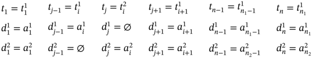
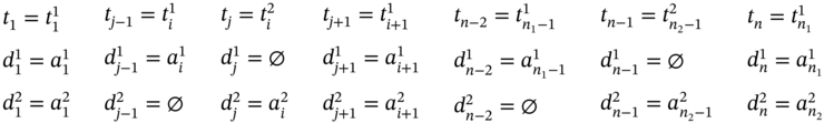
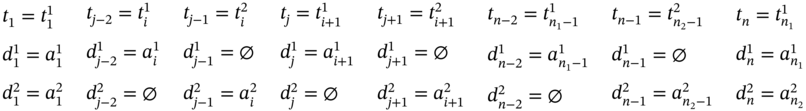
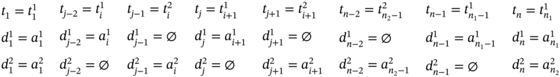
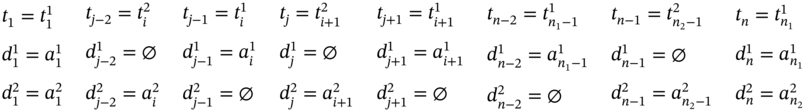
The rule for j index calculation is ![]() , where i ∈ [2…(n1 − 2)] and i is an even value (i mod 2 = 0). The total number of elements in each of the joint tuples, viz.,
, where i ∈ [2…(n1 − 2)] and i is an even value (i mod 2 = 0). The total number of elements in each of the joint tuples, viz., ![]() ,
, ![]() , and
, and ![]() , is
, is ![]() . If we consider the first and the last values of each joint tuple when
. If we consider the first and the last values of each joint tuple when ![]() and
and ![]() are connected with relation coincides with, we obtain the following:
are connected with relation coincides with, we obtain the following:
Similarly, if ![]() and
and ![]() , i mod 2 = 0,
, i mod 2 = 0, ![]() , and
, and ![]() , then the tuple value synchronization can be illustrated by Figure 5.2c. This case requires data synchronization defined in (5.57).
, then the tuple value synchronization can be illustrated by Figure 5.2c. This case requires data synchronization defined in (5.57).
If ![]() and
and ![]() (Figure 5.2d), ∀i ∈ [2…(n1 − 2)] such as i mod 2 = 0, then
(Figure 5.2d), ∀i ∈ [2…(n1 − 2)] such as i mod 2 = 0, then ![]() ,
, ![]() , and the tuple values of the multi‐image I are as follows:
, and the tuple values of the multi‐image I are as follows:
If ![]() and
and ![]() (Figure 5.2e), ∀i ∈ [2…(n1 − 2)] such as i mod 2 = 0, then j = 2i, n = 2(n1 − 1), and the tuple values of the multi‐image I can be obtained by using (5.59).
(Figure 5.2e), ∀i ∈ [2…(n1 − 2)] such as i mod 2 = 0, then j = 2i, n = 2(n1 − 1), and the tuple values of the multi‐image I can be obtained by using (5.59).

If ![]() ,
, ![]() , and
, and ![]() (Figure 5.2f), ∀i ∈ [2…(n1 − 2)] such as i mod 2 = 0, then j = 2i, n = 2(n1 − 1), and the tuple values of the multi‐image I can be defined as:
(Figure 5.2f), ∀i ∈ [2…(n1 − 2)] such as i mod 2 = 0, then j = 2i, n = 2(n1 − 1), and the tuple values of the multi‐image I can be defined as:
If ![]() ,
, ![]() , and
, and ![]() (Figure 5.2g), ∀i ∈ [2…(n1 − 2)] such as i mod 2 = 0, then
(Figure 5.2g), ∀i ∈ [2…(n1 − 2)] such as i mod 2 = 0, then ![]() ,
, ![]() , and the tuple values of the multi‐image I are as follows:
, and the tuple values of the multi‐image I are as follows:

If ![]() (Figure 5.2h), ∀i ∈ [2…(n1 − 2)] such as i mod 2 = 0, then j = 2i, n = 2(n1 − 1), and the tuple values of the multi‐image I are defined in (5.62).
(Figure 5.2h), ∀i ∈ [2…(n1 − 2)] such as i mod 2 = 0, then j = 2i, n = 2(n1 − 1), and the tuple values of the multi‐image I are defined in (5.62).
If ![]() and
and ![]() (Figure 5.2i), ∀i ∈ [2…(n1 − 2)] such as i mod 2 = 0, then j = 2i, n = 2(n1 − 1), and the tuple values of the multi‐image I are as follows:
(Figure 5.2i), ∀i ∈ [2…(n1 − 2)] such as i mod 2 = 0, then j = 2i, n = 2(n1 − 1), and the tuple values of the multi‐image I are as follows:

If ![]() and
and ![]() (Figure 5.2j), ∀i ∈ [2…(n1 − 2)] such as i mod 2 = 0, then
(Figure 5.2j), ∀i ∈ [2…(n1 − 2)] such as i mod 2 = 0, then ![]() ,
, ![]() , and the tuple values of the multi‐image I are defined in (5.64).
, and the tuple values of the multi‐image I are defined in (5.64).
If ![]() ,
, ![]() , and
, and ![]() (Figure 5.2k), ∀i ∈ [2…(n1 − 2)] such as i mod 2 = 0, then j = 2i, n = 2(n1 − 1), and the tuple values of the multi‐image I can be defined as follows:
(Figure 5.2k), ∀i ∈ [2…(n1 − 2)] such as i mod 2 = 0, then j = 2i, n = 2(n1 − 1), and the tuple values of the multi‐image I can be defined as follows:
If ![]() (Figure 5.2l), ∀i ∈ [2…(n1 − 2)] such as i mod 2 = 0, then
(Figure 5.2l), ∀i ∈ [2…(n1 − 2)] such as i mod 2 = 0, then ![]() ,
, ![]() , and the tuple values of the multi‐image I are as follows:
, and the tuple values of the multi‐image I are as follows:
If ![]() (Figure 5.2m), ∀i ∈ [2…(n1 − 2)] such as i mod 2 = 0, then j = 2i, n = 2(n1 − 1), and the tuple values of the multi‐image I are defined in (5.67).
(Figure 5.2m), ∀i ∈ [2…(n1 − 2)] such as i mod 2 = 0, then j = 2i, n = 2(n1 − 1), and the tuple values of the multi‐image I are defined in (5.67).
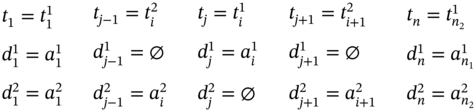
The second group of subcases for ![]() is when n1 is an odd value (n1 mod 2 ≠ 0) and
is when n1 is an odd value (n1 mod 2 ≠ 0) and ![]() , i.e.
, i.e. ![]() is equally frequent to
is equally frequent to ![]() ; it means that
; it means that ![]() (i.e. n1 = n2). Mutual alignment of i‐elements and (i + 1)‐elements in both data sequences for these subcases is similar to the subcases of the first group and, therefore, it is also illustrated in Figure 5.2. However, since n1 is an odd value, it complicates data synchronization because we need to analyze mutual alignment of
(i.e. n1 = n2). Mutual alignment of i‐elements and (i + 1)‐elements in both data sequences for these subcases is similar to the subcases of the first group and, therefore, it is also illustrated in Figure 5.2. However, since n1 is an odd value, it complicates data synchronization because we need to analyze mutual alignment of ![]() and
and ![]() as well.
as well.
If ![]() (Figure 5.2a), ∀i ∈ [1…n1], then the tuple values can be defined in the same way as it has been set in (5.54).
(Figure 5.2a), ∀i ∈ [1…n1], then the tuple values can be defined in the same way as it has been set in (5.54).
If ![]() ,
, ![]() (Figure 5.2b), ∀i ∈ [2…(n1 − 2)] such as i mod 2 = 0 and
(Figure 5.2b), ∀i ∈ [2…(n1 − 2)] such as i mod 2 = 0 and ![]() , then
, then ![]() ,
, ![]() and the tuple values of the multi‐image I can be defined as follows:
and the tuple values of the multi‐image I can be defined as follows:

If ![]() ,
, ![]() (Figure 5.2b), ∀i ∈ [2…(n1 − 2)] such as i mod 2 = 0, and
(Figure 5.2b), ∀i ∈ [2…(n1 − 2)] such as i mod 2 = 0, and ![]() , then
, then ![]() ,
, ![]() , and the tuple values of the multi‐image I are defined in (5.69).
, and the tuple values of the multi‐image I are defined in (5.69).
If ![]() ,
, ![]() (Figure 5.2b), ∀i ∈ [2…(n1 − 2)] such as i mod 2 = 0, and
(Figure 5.2b), ∀i ∈ [2…(n1 − 2)] such as i mod 2 = 0, and ![]() , then
, then ![]() ,
, ![]() , and the tuple values of the multi‐image I are as follows:
, and the tuple values of the multi‐image I are as follows:
If ![]() ,
, ![]() (Figure 5.2c), ∀i ∈ [2…(n1 − 2)] such as i mod 2 = 0, and
(Figure 5.2c), ∀i ∈ [2…(n1 − 2)] such as i mod 2 = 0, and ![]() , then
, then ![]() ,
, ![]() , and the tuple values of the multi‐image I are defined as:
, and the tuple values of the multi‐image I are defined as:
If ![]() ,
, ![]() (Figure 5.2c), ∀i ∈ [2…(n1 − 2)] such as i mod 2 = 0, and
(Figure 5.2c), ∀i ∈ [2…(n1 − 2)] such as i mod 2 = 0, and ![]() , then
, then ![]() ,
, ![]() , and the tuple values of the multi‐image I are stated in (5.72).
, and the tuple values of the multi‐image I are stated in (5.72).
If ![]() ,
, ![]() (Figure 5.2c), ∀i ∈ [2…(n1 − 2)] such as i mod 2 = 0, and
(Figure 5.2c), ∀i ∈ [2…(n1 − 2)] such as i mod 2 = 0, and ![]() , then
, then ![]() ,
, ![]() , and the tuple values of the multi‐image I are defined in (5.73).
, and the tuple values of the multi‐image I are defined in (5.73).
If ![]() ,
, ![]() (Figure 5.2d), ∀i ∈ [2…(n1 − 2)] such as i mod 2 = 0, and
(Figure 5.2d), ∀i ∈ [2…(n1 − 2)] such as i mod 2 = 0, and ![]() , then
, then ![]() ,
, ![]() , and the tuple values of the multi‐image I are as follows:
, and the tuple values of the multi‐image I are as follows:
If ![]() ,
, ![]() (Figure 5.2d), ∀i ∈ [2…(n1 − 2)] such as i mod 2 = 0, and
(Figure 5.2d), ∀i ∈ [2…(n1 − 2)] such as i mod 2 = 0, and ![]() , then
, then ![]() ,
, ![]() , and the tuple values of the multi‐image I can be defined as follows:
, and the tuple values of the multi‐image I can be defined as follows:
If ![]() ,
, ![]() (Figure 5.2d), ∀i ∈ [2…(n1 − 2)] such as i mod 2 = 0, and
(Figure 5.2d), ∀i ∈ [2…(n1 − 2)] such as i mod 2 = 0, and ![]() , then
, then ![]() ,
, ![]() , and the tuple values of the multi‐image I can be stated as follows:
, and the tuple values of the multi‐image I can be stated as follows:

If ![]() ,
, ![]() (Figure 5.2e), ∀i ∈ [2…(n1 − 2)] such as i mod 2 = 0, and
(Figure 5.2e), ∀i ∈ [2…(n1 − 2)] such as i mod 2 = 0, and ![]() , then j = 2i, n = 2n1 − 3, and the tuple values of the multi‐image I are as follows:
, then j = 2i, n = 2n1 − 3, and the tuple values of the multi‐image I are as follows:

If ![]() ,
, ![]() (Figure 5.2e), ∀i ∈ [2…(n1 − 2)] such as i mod 2 = 0, and
(Figure 5.2e), ∀i ∈ [2…(n1 − 2)] such as i mod 2 = 0, and ![]() , then j = 2i, n = 2(n1 − 1), and the tuple values of the multi‐image I are defined in (5.78).
, then j = 2i, n = 2(n1 − 1), and the tuple values of the multi‐image I are defined in (5.78).

If ![]() ,
, ![]() (Figure 5.2e), ∀i ∈ [2…(n1 − 2)] such as i mod 2 = 0, and
(Figure 5.2e), ∀i ∈ [2…(n1 − 2)] such as i mod 2 = 0, and ![]() , then j = 2i, n = 2(n1 − 1), and the tuple values of the multi‐image I are as follows:
, then j = 2i, n = 2(n1 − 1), and the tuple values of the multi‐image I are as follows:

If ![]() ,
, ![]() ,
, ![]() (Figure 5.2f), ∀i ∈ [2…(n1 − 2)] such as i mod 2 = 0, and
(Figure 5.2f), ∀i ∈ [2…(n1 − 2)] such as i mod 2 = 0, and ![]() , then j = 2i, n = 2n1 − 3, and the tuple values of the multi‐image I are defined in (5.80).
, then j = 2i, n = 2n1 − 3, and the tuple values of the multi‐image I are defined in (5.80).

If ![]() ,
, ![]() ,
, ![]() (Figure 5.2f), ∀i ∈ [2…(n1 − 2)] such as i mod 2 = 0, and
(Figure 5.2f), ∀i ∈ [2…(n1 − 2)] such as i mod 2 = 0, and ![]() , then j = 2i, n = 2(n1 − 1), and the tuple values of the multi‐image I can be obtained as follows:
, then j = 2i, n = 2(n1 − 1), and the tuple values of the multi‐image I can be obtained as follows:
If ![]() ,
, ![]() ,
, ![]() (Figure 5.2f), ∀i ∈ [2…(n1 − 2)] such as i mod 2 = 0, and
(Figure 5.2f), ∀i ∈ [2…(n1 − 2)] such as i mod 2 = 0, and ![]() , then j = 2i, n = 2(n1 − 1), and the tuple values of the multi‐image I are defined in (5.82).
, then j = 2i, n = 2(n1 − 1), and the tuple values of the multi‐image I are defined in (5.82).
If ![]() ,
, ![]() ,
, ![]() (Figure 5.2g), ∀i ∈ [2…(n1 − 2)] such as i mod 2 = 0, and
(Figure 5.2g), ∀i ∈ [2…(n1 − 2)] such as i mod 2 = 0, and ![]() , then
, then ![]() ,
, ![]() , and the tuple values of the multi‐image I are as follows:
, and the tuple values of the multi‐image I are as follows:

If ![]() ,
, ![]() ,
, ![]() (Figure 5.2g), ∀i ∈ [2…(n1 − 2)] such as i mod 2 = 0, and
(Figure 5.2g), ∀i ∈ [2…(n1 − 2)] such as i mod 2 = 0, and ![]() , then
, then ![]() ,
, ![]() , and the tuple values of the multi‐image I can be obtained by using (5.84).
, and the tuple values of the multi‐image I can be obtained by using (5.84).

If ![]() ,
, ![]() ,
, ![]() (Figure 5.2g), ∀i ∈ [2…(n1 − 2)] such as i mod 2 = 0, and
(Figure 5.2g), ∀i ∈ [2…(n1 − 2)] such as i mod 2 = 0, and ![]() , then
, then ![]() ,
, ![]() , and the tuple values of the multi‐image I are as follows:
, and the tuple values of the multi‐image I are as follows:

If ![]() (Figure 5.2h), ∀i ∈ [2…(n1 − 2)] such as i mod 2 = 0 and
(Figure 5.2h), ∀i ∈ [2…(n1 − 2)] such as i mod 2 = 0 and ![]() , then j = 2i, n = 2n1 − 3, and the tuple values of the multi‐image I can be found as defined in (5.86).
, then j = 2i, n = 2n1 − 3, and the tuple values of the multi‐image I can be found as defined in (5.86).
If ![]() (Figure 5.2h), ∀i ∈ [2…(n1 − 2)] such as i mod 2 = 0, and
(Figure 5.2h), ∀i ∈ [2…(n1 − 2)] such as i mod 2 = 0, and ![]() , then j = 2i, n = 2(n1 − 1), and the tuple values of the multi‐image I are stated as follows:
, then j = 2i, n = 2(n1 − 1), and the tuple values of the multi‐image I are stated as follows:
If ![]() (Figure 5.2h), ∀i ∈ [2…(n1 − 2)] such as i mod 2 = 0 and
(Figure 5.2h), ∀i ∈ [2…(n1 − 2)] such as i mod 2 = 0 and ![]() , then j = 2i, n = 2(n1 − 1), and the tuple values of the multi‐image I can be defined as:
, then j = 2i, n = 2(n1 − 1), and the tuple values of the multi‐image I can be defined as:

If ![]() ,
, ![]() (Figure 5.2i), ∀i ∈ [2…(n1 − 2)] such as i mod 2 = 0, and
(Figure 5.2i), ∀i ∈ [2…(n1 − 2)] such as i mod 2 = 0, and ![]() , then j = 2i, n = 2n1 − 3, and the tuple values of the multi‐image I are as follows:
, then j = 2i, n = 2n1 − 3, and the tuple values of the multi‐image I are as follows:

If ![]() ,
, ![]() (Figure 5.2i), ∀i ∈ [2…(n1 − 2)] such as i mod 2 = 0, and
(Figure 5.2i), ∀i ∈ [2…(n1 − 2)] such as i mod 2 = 0, and ![]() , then j = 2i, n = 2(n1 − 1), and the tuple values of the multi‐image I are defined as:
, then j = 2i, n = 2(n1 − 1), and the tuple values of the multi‐image I are defined as:
If ![]() ,
, ![]() (Figure 5.2i), ∀i ∈ [2…(n1 − 2)] such as i mod 2 = 0, and
(Figure 5.2i), ∀i ∈ [2…(n1 − 2)] such as i mod 2 = 0, and ![]() , then j = 2i, n = 2(n1 − 1), and the tuple values of the multi‐image I are stated in (5.91).
, then j = 2i, n = 2(n1 − 1), and the tuple values of the multi‐image I are stated in (5.91).
If ![]() ,
, ![]() (Figure 5.2j), ∀i ∈ [2…(n1 − 2)] such as i mod 2 = 0, and
(Figure 5.2j), ∀i ∈ [2…(n1 − 2)] such as i mod 2 = 0, and ![]() , then
, then ![]() ,
, ![]() , and the tuple values of the multi‐image I are defined in (5.92).
, and the tuple values of the multi‐image I are defined in (5.92).
If ![]() ,
, ![]() (Figure 5.2j), ∀i ∈ [2…(n1 − 2)] such as i mod 2 = 0, and
(Figure 5.2j), ∀i ∈ [2…(n1 − 2)] such as i mod 2 = 0, and ![]() , then
, then ![]() ,
, ![]() , and the tuple values of the multi‐image I are as follows:
, and the tuple values of the multi‐image I are as follows:
If ![]() ,
, ![]() (Figure 5.2j), ∀i ∈ [2…(n1 − 2)] such as i mod 2 = 0, and
(Figure 5.2j), ∀i ∈ [2…(n1 − 2)] such as i mod 2 = 0, and ![]() , then
, then ![]() ,
, ![]() , and the tuple values of the multi‐image I can be defined as:
, and the tuple values of the multi‐image I can be defined as:
If ![]() ,
, ![]() ,
, ![]() (Figure 5.2k), ∀i ∈ [2…(n1 − 2)] such as i mod 2 = 0, and
(Figure 5.2k), ∀i ∈ [2…(n1 − 2)] such as i mod 2 = 0, and ![]() , then j = 2i, n = 2n1 − 3, and the tuple values of the multi‐image I are defined in (5.95).
, then j = 2i, n = 2n1 − 3, and the tuple values of the multi‐image I are defined in (5.95).
If ![]() ,
, ![]() ,
, ![]() (Figure 5.2k), ∀i ∈ [2…(n1 − 2)] such as i mod 2 = 0, and
(Figure 5.2k), ∀i ∈ [2…(n1 − 2)] such as i mod 2 = 0, and ![]() , then j = 2i, n = 2(n1 − 1), and the tuple values of the multi‐image I are as follows:
, then j = 2i, n = 2(n1 − 1), and the tuple values of the multi‐image I are as follows:
If ![]() ,
, ![]() ,
, ![]() (Figure 5.2k), ∀i ∈ [2…(n1 − 2)] such as i mod 2 = 0, and
(Figure 5.2k), ∀i ∈ [2…(n1 − 2)] such as i mod 2 = 0, and ![]() , then j = 2i, n = 2(n1 − 1), and the tuple values of the multi‐image I can be obtained as follows:
, then j = 2i, n = 2(n1 − 1), and the tuple values of the multi‐image I can be obtained as follows:

If ![]() (Figure 5.2l), ∀i ∈ [2…(n1 − 2)] such as i mod 2 = 0 and
(Figure 5.2l), ∀i ∈ [2…(n1 − 2)] such as i mod 2 = 0 and ![]() , then
, then ![]() ,
, ![]() , and the tuple values of the multi‐image I are defined in (5.98).
, and the tuple values of the multi‐image I are defined in (5.98).
If ![]() (Figure 5.2l), ∀i ∈ [2…(n1 − 2)] such as i mod 2 = 0, and
(Figure 5.2l), ∀i ∈ [2…(n1 − 2)] such as i mod 2 = 0, and ![]() , then
, then ![]() ,
, ![]() , and the tuple values of the multi‐image I are as follows:
, and the tuple values of the multi‐image I are as follows:

If ![]() (Figure 5.2l), ∀i ∈ [2…(n1 − 2)] such as i mod 2 = 0, and
(Figure 5.2l), ∀i ∈ [2…(n1 − 2)] such as i mod 2 = 0, and ![]() , then
, then ![]() ,
, ![]() , and the tuple values of the multi‐image I can be obtained by using (5.100).
, and the tuple values of the multi‐image I can be obtained by using (5.100).
If ![]() (Figure 5.2m), ∀i ∈ [2…(n1 − 2)] such as i mod 2 = 0, and
(Figure 5.2m), ∀i ∈ [2…(n1 − 2)] such as i mod 2 = 0, and ![]() , then j = 2i, n = 2n1 − 3, and the tuple values of the multi‐image I are as follows:
, then j = 2i, n = 2n1 − 3, and the tuple values of the multi‐image I are as follows:

If ![]() (Figure 5.2m), ∀i ∈ [2…(n1 − 2)] such as i mod 2 = 0, and
(Figure 5.2m), ∀i ∈ [2…(n1 − 2)] such as i mod 2 = 0, and ![]() , then j = 2i, n = 2(n1 − 1), and the tuple values of the multi‐image I can be found as defined in (5.102).
, then j = 2i, n = 2(n1 − 1), and the tuple values of the multi‐image I can be found as defined in (5.102).
If ![]() (Figure 5.2m), ∀i ∈ [2…(n1 − 2)] such as i mod 2 = 0 and
(Figure 5.2m), ∀i ∈ [2…(n1 − 2)] such as i mod 2 = 0 and ![]() , then j = 2i, n = 2(n1 − 1), and the tuple values of the multi‐image I are as follows:
, then j = 2i, n = 2(n1 − 1), and the tuple values of the multi‐image I are as follows:
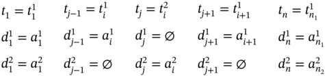
The third group of subcases (Figure 5.3) for ![]() is when
is when ![]() , i.e.
, i.e. ![]() is rarer than
is rarer than ![]() ; it means that
; it means that ![]() . Because ratio R between
. Because ratio R between ![]() and
and ![]() can be various, let us assume that for every i‐element in
can be various, let us assume that for every i‐element in ![]() , there are two elements in
, there are two elements in ![]() , except
, except ![]() and
and ![]() , which coincide with
, which coincide with ![]() and
and ![]() , respectively (Figure 5.3). It means that n2 mod 2 = 0 and
, respectively (Figure 5.3). It means that n2 mod 2 = 0 and ![]() .
.
If ![]() (Figure 5.3a), ∀i ∈ [2…(n2 − 2)] such as i mod 2 = 0, then n = n2 and the tuple values of the multi‐image I can be defined as:
(Figure 5.3a), ∀i ∈ [2…(n2 − 2)] such as i mod 2 = 0, then n = n2 and the tuple values of the multi‐image I can be defined as:
If ![]() (Figure 5.3b), ∀i ∈ [2…(n2 − 2)] such as i mod 2 = 0, then
(Figure 5.3b), ∀i ∈ [2…(n2 − 2)] such as i mod 2 = 0, then ![]() ,
, ![]() , and the tuple values of the multi‐image I are as follows:
, and the tuple values of the multi‐image I are as follows:
If ![]() (Figure 5.3c), ∀i ∈ [2…(n2 − 2)] such as i mod 2 = 0, then n = n2 and the tuple values of the multi‐image I are defined in (5.106).
(Figure 5.3c), ∀i ∈ [2…(n2 − 2)] such as i mod 2 = 0, then n = n2 and the tuple values of the multi‐image I are defined in (5.106).
If ![]() (Figure 5.3d), ∀i ∈ [2…(n2 − 2)] such as i mod 2 = 0, then
(Figure 5.3d), ∀i ∈ [2…(n2 − 2)] such as i mod 2 = 0, then ![]() ,
, ![]() , and the tuple values of the multi‐image I are as follows:
, and the tuple values of the multi‐image I are as follows:
If ![]() and
and ![]() (Figure 5.3e), ∀i ∈ [2…(n2 − 2)] such as i mod 2 = 0, then
(Figure 5.3e), ∀i ∈ [2…(n2 − 2)] such as i mod 2 = 0, then ![]() ,
, ![]() , and the tuple values of the multi‐image I are defined as:
, and the tuple values of the multi‐image I are defined as:
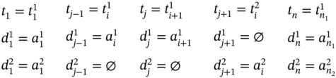
The forth group of subcases for ![]() is when
is when ![]() , i.e.
, i.e. ![]() is thicker than
is thicker than ![]() ; it means that
; it means that ![]() . Similar to the third group (
. Similar to the third group (![]() ), ratio R between
), ratio R between ![]() and
and ![]() can vary. Thus, we assume that for every i‐element in
can vary. Thus, we assume that for every i‐element in ![]() , there are two elements in
, there are two elements in ![]() , except
, except ![]() and
and ![]() , which coincide with
, which coincide with ![]() and
and ![]() , respectively (Figure 5.4). It means that n1 mod 2 = 0 and
, respectively (Figure 5.4). It means that n1 mod 2 = 0 and ![]() .
.
If ![]() (Figure 5.4a), ∀i ∈ [2…(n1 − 2)] such as i mod 2 = 0, then n = n1 and the tuple values of the multi‐image I can be defined as:
(Figure 5.4a), ∀i ∈ [2…(n1 − 2)] such as i mod 2 = 0, then n = n1 and the tuple values of the multi‐image I can be defined as:

If ![]() (Figure 5.4b), ∀i ∈ [2…(n1 − 2)] such as i mod 2 = 0, then
(Figure 5.4b), ∀i ∈ [2…(n1 − 2)] such as i mod 2 = 0, then ![]() ,
, ![]() , and the tuple values of the multi‐image I are as follows:
, and the tuple values of the multi‐image I are as follows:

If ![]() and
and ![]() (Figure 5.4c), ∀i ∈ [2…(n1 − 2)] such as i mod 2 = 0, then
(Figure 5.4c), ∀i ∈ [2…(n1 − 2)] such as i mod 2 = 0, then ![]() ,
, ![]() , and the tuple values of the multi‐image I are defined in (5.111).
, and the tuple values of the multi‐image I are defined in (5.111).
If ![]() (Figure 5.4d), ∀i ∈ [2…(n1 − 2)] such as i mod 2 = 0, then
(Figure 5.4d), ∀i ∈ [2…(n1 − 2)] such as i mod 2 = 0, then ![]() ,
, ![]() , and the tuple values of the multi‐image I are as follows:
, and the tuple values of the multi‐image I are as follows:
If ![]() (Figure 5.4e), ∀i ∈ [2…(n1 − 2)] such as i mod 2 = 0, then n = n1 and the tuple values of the multi‐image I are defined in (5.113).
(Figure 5.4e), ∀i ∈ [2…(n1 − 2)] such as i mod 2 = 0, then n = n1 and the tuple values of the multi‐image I are defined in (5.113).

Thus, we presented all possible subcases for the relation coincides with.
The case, which is more general than defined above, is when the same number of measurements of both ![]() and
and ![]() have been fulfilled in the same period of time from the moment α to the moment β but not simultaneously. It means that
have been fulfilled in the same period of time from the moment α to the moment β but not simultaneously. It means that ![]() and
and ![]() are connected by the relation between defined in (5.49). The difference between the relations coincides with and between consists in defining the first and the last values of tuples in a multi‐image. The first values of tuples are to be defined based on comparison of
are connected by the relation between defined in (5.49). The difference between the relations coincides with and between consists in defining the first and the last values of tuples in a multi‐image. The first values of tuples are to be defined based on comparison of ![]() and
and ![]() :
:

The last values of tuples are to be defined based on comparison of ![]() and
and ![]() :
:

The rest of tuple elements are to be defined in the same way as stated in (5.54)–(5.113).
The case, when measuring of ![]() forestalls measuring of
forestalls measuring of ![]() , means that
, means that ![]() and
and ![]() are connected by the relation is before defined in (5.37). Thus, if
are connected by the relation is before defined in (5.37). Thus, if ![]() , then ∀i1 ∈ [1…n1], ∀i2 ∈ [1…n2]:
, then ∀i1 ∈ [1…n1], ∀i2 ∈ [1…n2]:
The case, when measuring of ![]() succeeds measuring of
succeeds measuring of ![]() , means that
, means that ![]() and
and ![]() are connected by the relation is after defined in (5.38). Thus, if
are connected by the relation is after defined in (5.38). Thus, if ![]() , then ∀i1 ∈ [1…n1], ∀i2 ∈ [1…n2]:
, then ∀i1 ∈ [1…n1], ∀i2 ∈ [1…n2]:
The case, when measuring of ![]() forestalls measuring of
forestalls measuring of ![]() , but measuring of the last value of
, but measuring of the last value of ![]() coincides with measuring of the first value of
coincides with measuring of the first value of ![]() , means that
, means that ![]() and
and ![]() are connected by the relation meets defined in (5.39). Thus, if
are connected by the relation meets defined in (5.39). Thus, if ![]() then ∀i1 ∈ [1…(n1 − 1)], ∀i2 ∈ [2…n2]:
then ∀i1 ∈ [1…(n1 − 1)], ∀i2 ∈ [2…n2]:
The case, when measuring of ![]() succeeds measuring of
succeeds measuring of ![]() , but measuring of the first value of
, but measuring of the first value of ![]() coincides with measuring of the last value of
coincides with measuring of the last value of ![]() , means that
, means that ![]() and
and ![]() are connected by the relation is met by defined in (5.40). Thus, if
are connected by the relation is met by defined in (5.40). Thus, if ![]() , then ∀i1 ∈ [2…n1], ∀i2 ∈ [1…(n2 − 1)]:
, then ∀i1 ∈ [2…n1], ∀i2 ∈ [1…(n2 − 1)]:
The case, when measuring of ![]() forestalls measuring of
forestalls measuring of ![]() , but measuring of K last values of
, but measuring of K last values of ![]() coincides with measuring of K first values of
coincides with measuring of K first values of ![]() , means that
, means that ![]() and
and ![]() are connected by the relation overlaps defined in (5.41). Thus, if
are connected by the relation overlaps defined in (5.41). Thus, if ![]() , then ∀i1 ∈ [1…(n1 − K)], ∀i2 ∈ [(K + 1)…n2], ∀k ∈ [1…K]:
, then ∀i1 ∈ [1…(n1 − K)], ∀i2 ∈ [(K + 1)…n2], ∀k ∈ [1…K]:
The case, when measuring of ![]() succeeds measuring of
succeeds measuring of ![]() , but measuring of K first values of
, but measuring of K first values of ![]() coincides with measuring of K last values of
coincides with measuring of K last values of ![]() , means that
, means that ![]() and
and ![]() are connected by the relation is overlapped by defined in (5.42). Thus, if
are connected by the relation is overlapped by defined in (5.42). Thus, if ![]() , then ∀i1 ∈ [(K + 1)…n1], ∀i2 ∈ [1…(n2 − K)], and ∀k ∈ [1…K]:
, then ∀i1 ∈ [(K + 1)…n1], ∀i2 ∈ [1…(n2 − K)], and ∀k ∈ [1…K]:

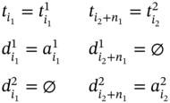
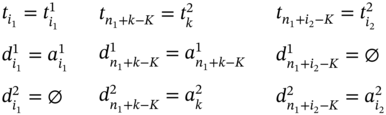
The case, when measuring of ![]() starts later and at the same time it finishes earlier than measuring of
starts later and at the same time it finishes earlier than measuring of ![]() does, means that
does, means that ![]() and
and ![]() are connected by the relation during defined in (5.43). Thus, if
are connected by the relation during defined in (5.43). Thus, if ![]() , therefore,
, therefore, ![]() such as
such as ![]() ,
, ![]() , and
, and ![]() . Then, ∀ k1 ∈ [1…K1], ∀ k2 ∈ [K2…n2] such as
. Then, ∀ k1 ∈ [1…K1], ∀ k2 ∈ [K2…n2] such as ![]() and
and ![]() , we can define the first values
, we can define the first values ![]() (
(![]() ),
), ![]() ,
, ![]() , and the last values
, and the last values ![]() (
(![]() ),
), ![]() ,
, ![]() of the resulting tuples
of the resulting tuples ![]() ,
, ![]() , and
, and ![]() as defined in (5.122). The rest of tuple elements (
as defined in (5.122). The rest of tuple elements (![]() ,
, ![]() ,
, ![]() ) of the resulting tuples
) of the resulting tuples ![]() ,
, ![]() , and
, and ![]() can be obtained accordingly to subcases defined in (5.54)–(5.115). Then, the length of the resulting tuple
can be obtained accordingly to subcases defined in (5.54)–(5.115). Then, the length of the resulting tuple ![]() is n = K1 + m + n2 − K2 + 1, where m is the length of the tuple obtained as a result of synchronization of tuples
is n = K1 + m + n2 − K2 + 1, where m is the length of the tuple obtained as a result of synchronization of tuples ![]() and
and ![]() .
.

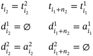
The case, when measuring of ![]() starts earlier and at the same time it finishes later than measuring of
starts earlier and at the same time it finishes later than measuring of ![]() does, means that
does, means that ![]() and
and ![]() are connected by the relation contains defined in (5.44). Thus, if
are connected by the relation contains defined in (5.44). Thus, if ![]() , therefore,
, therefore, ![]() such as
such as ![]() ,
, ![]() , and
, and ![]() . Then, ∀ k1 ∈ [1…K1] and ∀ k2 ∈ [K2…n1] such as
. Then, ∀ k1 ∈ [1…K1] and ∀ k2 ∈ [K2…n1] such as ![]() and
and ![]() , we can define the first values
, we can define the first values ![]() (
(![]() ),
), ![]() , and
, and ![]() and the last values
and the last values ![]() (
(![]() ),
), ![]() , and
, and ![]() of the resulting tuples
of the resulting tuples ![]() ,
, ![]() , and
, and ![]() as defined in (5.123). The rest of tuple elements (
as defined in (5.123). The rest of tuple elements (![]() ,
, ![]() ,
, ![]() ) of the resulting tuples
) of the resulting tuples ![]() ,
, ![]() , and
, and ![]() can be obtained accordingly to subcases defined in (5.54)–(5.115). Then, the length of the resulting tuple
can be obtained accordingly to subcases defined in (5.54)–(5.115). Then, the length of the resulting tuple ![]() is n = K1 + m + n1 − K2 + 1, where m is the length of the tuple obtained as a result of synchronization of tuples
is n = K1 + m + n1 − K2 + 1, where m is the length of the tuple obtained as a result of synchronization of tuples ![]() and
and ![]() .
.

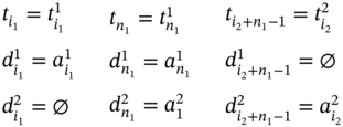
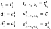
The case, when measuring of both ![]() and
and ![]() start simultaneously, but measuring of
start simultaneously, but measuring of ![]() finishes earlier than measuring of
finishes earlier than measuring of ![]() does, means that
does, means that ![]() and
and ![]() are connected by the relation starts defined in (5.45). Thus, if
are connected by the relation starts defined in (5.45). Thus, if ![]() , therefore,
, therefore, ![]() such as
such as ![]() and
and ![]() . Then, ∀k2 ∈ [K…n2] such as
. Then, ∀k2 ∈ [K…n2] such as ![]() , we can define the first value t1(
, we can define the first value t1(![]() ),
), ![]() , and
, and ![]() and the last values
and the last values ![]() (
(![]() ),
), ![]() , and
, and ![]() of the resulting tuples
of the resulting tuples ![]() ,
, ![]() , and
, and ![]() as defined in (5.124). The rest of tuple elements (
as defined in (5.124). The rest of tuple elements (![]() ,
, ![]() ,
, ![]() , and ∀k1 ∈ [2…m], where m is the length of the tuple obtained as a result of synchronization of tuples
, and ∀k1 ∈ [2…m], where m is the length of the tuple obtained as a result of synchronization of tuples ![]() and
and ![]() ) of the resulting tuples
) of the resulting tuples ![]() ,
, ![]() , and
, and ![]() can be obtained accordingly to subcases defined in (5.54)–(5.115). Then, the length of the resulting tuple
can be obtained accordingly to subcases defined in (5.54)–(5.115). Then, the length of the resulting tuple ![]() is n = m + n2 − K + 1.
is n = m + n2 − K + 1.
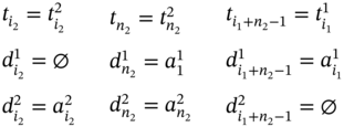
The case, when measuring of both ![]() and
and ![]() start simultaneously, but measuring of
start simultaneously, but measuring of ![]() finishes later than measuring of
finishes later than measuring of ![]() does, means that
does, means that ![]() and
and ![]() are connected by the relation is started by defined in (5.46). Thus, if
are connected by the relation is started by defined in (5.46). Thus, if ![]() , therefore,
, therefore, ![]() such as
such as ![]() and
and ![]() . Then, ∀k2 ∈ [K…n1] such as
. Then, ∀k2 ∈ [K…n1] such as ![]() , we can define the first value t1(
, we can define the first value t1(![]() ),
), ![]() ,
, ![]() , and the last values
, and the last values ![]() (
(![]() ),
), ![]() , and
, and ![]() of the resulting tuples
of the resulting tuples ![]() ,
, ![]() , and
, and ![]() as defined in (5.125). The rest of tuple elements (
as defined in (5.125). The rest of tuple elements (![]() ,
, ![]() ,
, ![]() , and ∀ k1 ∈ [2…m], where m is the length of the tuple obtained as a result of synchronization of tuples
, and ∀ k1 ∈ [2…m], where m is the length of the tuple obtained as a result of synchronization of tuples ![]() and
and ![]() ) of the resulting tuples
) of the resulting tuples ![]() ,
, ![]() , and
, and ![]() can be obtained accordingly to subcases defined in (5.54)–(5.115). Then, the length of the resulting tuple
can be obtained accordingly to subcases defined in (5.54)–(5.115). Then, the length of the resulting tuple ![]() is n = m + n1 − K + 1.
is n = m + n1 − K + 1.
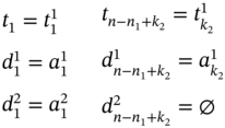
The case, when measuring of both ![]() and
and ![]() finish simultaneously, but measuring of
finish simultaneously, but measuring of ![]() starts later than measuring of
starts later than measuring of ![]() does, means that
does, means that ![]() and
and ![]() are connected by the relation finishes defined in (5.47). Thus, if
are connected by the relation finishes defined in (5.47). Thus, if ![]() , therefore,
, therefore, ![]() such as
such as ![]() and
and ![]() . Then, ∀ k1 ∈ [1…K], such as
. Then, ∀ k1 ∈ [1…K], such as ![]() , we can define the first values
, we can define the first values ![]() (
(![]() ),
), ![]() , and
, and ![]() and the last value tn (
and the last value tn (![]() ),
), ![]() , and
, and ![]() of the resulting tuples
of the resulting tuples ![]() ,
, ![]() , and
, and ![]() as defined in (5.126). The rest of tuple elements (
as defined in (5.126). The rest of tuple elements (![]() ,
, ![]() ,
, ![]() , and ∀k2 ∈ [(K + 1)…(n − 1)], where the length of the resulting tuple
, and ∀k2 ∈ [(K + 1)…(n − 1)], where the length of the resulting tuple ![]() is n = K + m; m is the length of the tuple obtained as a result of synchronization of tuples
is n = K + m; m is the length of the tuple obtained as a result of synchronization of tuples ![]() and
and ![]() ) of the resulting tuples
) of the resulting tuples ![]() ,
, ![]() , and
, and ![]() can be obtained accordingly to subcases defined in (5.54)–(5.115).
can be obtained accordingly to subcases defined in (5.54)–(5.115).

The case, when measuring of both ![]() and
and ![]() finish simultaneously, but measuring of
finish simultaneously, but measuring of ![]() starts earlier than measuring of
starts earlier than measuring of ![]() does, means that
does, means that ![]() and
and ![]() are connected by the relation is finished by defined in (5.48). Thus, if
are connected by the relation is finished by defined in (5.48). Thus, if ![]() , therefore,
, therefore, ![]() such as
such as ![]() and
and ![]() . Then, ∀k1 ∈ [1…K], such as
. Then, ∀k1 ∈ [1…K], such as ![]() , we can define the first values
, we can define the first values ![]() (
(![]() ),
), ![]() , and
, and ![]() and the last value tn (
and the last value tn (![]() ),
), ![]() , and
, and ![]() of the resulting tuples
of the resulting tuples ![]() ,
, ![]() , and
, and ![]() as defined in (5.127). The rest of tuple elements (
as defined in (5.127). The rest of tuple elements (![]() ,
, ![]() , and
, and ![]() , ∀k2 ∈ [(K + 1)…(n − 1)], where the length of the resulting tuple
, ∀k2 ∈ [(K + 1)…(n − 1)], where the length of the resulting tuple ![]() is n = K + m; m is the length of the tuple obtained as a result of synchronization of tuples
is n = K + m; m is the length of the tuple obtained as a result of synchronization of tuples ![]() and
and ![]() ) of the resulting tuples
) of the resulting tuples ![]() ,
, ![]() , and
, and ![]() can be obtained accordingly to subcases defined in (5.54)–(5.115).
can be obtained accordingly to subcases defined in (5.54)–(5.115).

As one can see, in the case of crisp time value processing, there is a great number of cases for data synchronization. Thus, in applications where the crisp time values are not strictly required, it is reasonable to use fuzzy synchronization.
5.6 Fuzzy Synchronization
For fuzzy data synchronization of multi‐images, we need fuzzy equivalents of temporal relations defined by (5.36)–(5.49). There is a number of works on this topic, in particular, [11,14–18]. In this research, we apply the approach formulated in [11,18]. Let us present it in detail.
The degree ![]() to which the beginning of
to which the beginning of ![]() is approximately α(α ∈ ℝ) time units before the beginning of
is approximately α(α ∈ ℝ) time units before the beginning of ![]() , where β (β ≥ 0) indicates a degree of tolerance, is a fuzzification generalization of strict inequality
, where β (β ≥ 0) indicates a degree of tolerance, is a fuzzification generalization of strict inequality ![]() ; it is defined as follows:
; it is defined as follows:
where the operation ∘T means composition of fuzzy relations as defined in (5.129); the operation ⊳I means superproduct as defined in (5.130) according to [19]; Tw is Łukasiewicz t‐norm defined in (5.131); ![]() is a Łukasiewicz implicator defined in (5.132);
is a Łukasiewicz implicator defined in (5.132); ![]() is the fuzzy relation between time points
is the fuzzy relation between time points ![]() and
and ![]() defined in (5.133).
defined in (5.133).
The sup‐T composition of fuzzy relations is defined as:
where R1 is a fuzzy relation from a set X to a set Y; R2 is a fuzzy relation from a set Y to a set Z; x ∈ X, y ∈ Y, z ∈ Z.
The I‐superproduct of fuzzy relations is defined as:
The Łukasiewicz triangular norm and its corresponding implicator are given as:
where a, b ∈ [0, 1].
The fuzzy relation ![]() models a metric constraint between time points and is given as:
models a metric constraint between time points and is given as:

where α is the distance (in time units) between ![]() and
and ![]() and β is the degree of tolerance.
and β is the degree of tolerance.
The degree ![]() to which the beginning of
to which the beginning of ![]() is approximately α time units before or the same time as the beginning of
is approximately α time units before or the same time as the beginning of ![]() is a generalization of the nonstrict inequality
is a generalization of the nonstrict inequality ![]() ; it is defined as follows:
; it is defined as follows:
The degree ![]() to which the end of
to which the end of ![]() is approximately α time units before the end of
is approximately α time units before the end of ![]() is a generalization of the strict inequality
is a generalization of the strict inequality ![]() ; it is defined as follows:
; it is defined as follows:
where the operation ⊲I means subproduct as defined in (5.136) according to [19].
The degree ![]() to which the end of
to which the end of ![]() is approximately α time units before or the same time as the end of
is approximately α time units before or the same time as the end of ![]() is a generalization of the nonstrict inequality
is a generalization of the nonstrict inequality ![]() ; it is defined as follows:
; it is defined as follows:
The degree ![]() to which the beginning of
to which the beginning of ![]() is approximately α time units before the end of
is approximately α time units before the end of ![]() is a generalization of the strict inequality
is a generalization of the strict inequality ![]() ; it is defined as follows:
; it is defined as follows:
The degree ![]() to which the beginning of
to which the beginning of ![]() is approximately α time units before or the same time as the end of
is approximately α time units before or the same time as the end of ![]() is a generalization of the nonstrict inequality
is a generalization of the nonstrict inequality ![]() ; it is defined as follows:
; it is defined as follows:
The degree ![]() to which the end of
to which the end of ![]() is approximately α time units before the beginning of
is approximately α time units before the beginning of ![]() is a generalization of the strict inequality
is a generalization of the strict inequality ![]() ; it is defined as follows:
; it is defined as follows:
The degree ![]() to which the end of
to which the end of ![]() is approximately α time units before or the same time as the beginning of
is approximately α time units before or the same time as the beginning of ![]() is a generalization of the nonstrict inequality
is a generalization of the nonstrict inequality ![]() ; it is defined as follows:
; it is defined as follows:
As one can see in Section 5.5, crisp data synchronization in the case when ![]() is quite complicated because of many subcases. We can simplify data synchronization if we consider the degree of closeness between time moments
is quite complicated because of many subcases. We can simplify data synchronization if we consider the degree of closeness between time moments ![]() and
and ![]() . Such degree can be estimated as
. Such degree can be estimated as ![]() . Let us prove that if Δt is a minimal distance between
. Let us prove that if Δt is a minimal distance between ![]() and
and ![]() (we assume Δt as a time measurement error), then
(we assume Δt as a time measurement error), then ![]() and, thus,
and, thus, ![]() and
and ![]() can be considered as one fuzzy moment of time
can be considered as one fuzzy moment of time ![]() .
.
According to (5.140), ![]() . From expressions (5.130) and (5.136), we obtain the following:
. From expressions (5.130) and (5.136), we obtain the following:
Taking into account (5.132), we have:
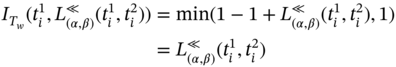
Similarly,
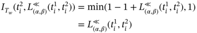
Thus, we can rewrite (5.142) as follows:
Then, we have from (5.133) that:
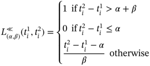
Since ![]() , we have
, we have ![]() in (5.146) because Δt is a time measurement error, i.e. it is the least possible distance between
in (5.146) because Δt is a time measurement error, i.e. it is the least possible distance between ![]() and
and ![]() .
.
Thus, ![]() and therefore
and therefore ![]() . From practical point of view, it means that if there is a time measurement error in two time value sequences
. From practical point of view, it means that if there is a time measurement error in two time value sequences ![]() and
and ![]() (actually, it can happen in many cases if the measurements are taken simultaneously but by different executors, e.g. atmosphere pressure is being measured in one research unit and the sun's radiation is being measured by another research unit), we may neglect this time measurement error.
(actually, it can happen in many cases if the measurements are taken simultaneously but by different executors, e.g. atmosphere pressure is being measured in one research unit and the sun's radiation is being measured by another research unit), we may neglect this time measurement error.
Now let the distance between time moments ![]() and
and ![]() exceed Δt and be equal to α. Then, in (5.146), we have
exceed Δt and be equal to α. Then, in (5.146), we have ![]() ; thus,
; thus, ![]() and therefore
and therefore ![]() . Thus, the conclusion is that we again can consider these two time moments
. Thus, the conclusion is that we again can consider these two time moments ![]() and
and ![]() as one fuzzy moment of time
as one fuzzy moment of time ![]() .
.
Let us consider different cases (Figure 5.5) for α between neighboring values in ![]() and
and ![]() when
when ![]() in order to simplify data value synchronization defined by (5.54)–(5.113). Let α1 be a distance between
in order to simplify data value synchronization defined by (5.54)–(5.113). Let α1 be a distance between ![]() and
and ![]() , let α2 be a distance between
, let α2 be a distance between ![]() and
and ![]() , and let α3 be a distance between
, and let α3 be a distance between ![]() and
and ![]() . Besides, let α be a minimal distance between such
. Besides, let α be a minimal distance between such ![]() and
and ![]() that we can consider them as one vague time moment to be presented as one fuzzy value
that we can consider them as one vague time moment to be presented as one fuzzy value ![]() in the time tuple of a multi‐image.
in the time tuple of a multi‐image.
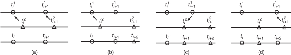
Figure 5.5 Fuzzy synchronization cases.  and
and  are elements of the time tuple
  ;
;  and
and  are elements of the time tuple
  ; tj, tj + 1, and tj + 2 are elements of the synchronized time tuple
  . For two measurement processes: (a) measurements of both parameters are almost simultaneous at the current and the next moments of time; (b) the current measurements of both parameters are almost simultaneous; (c) the next measurement of the 1st parameter and the current measurement of the 2nd parameter are almost simultaneous; (d) the next measurements of both parameters are almost simultaneous.
If both α1 < α and α3 < α are true (Figure 5.5a), then regardless of the value of α2, the data synchronization can be simplified to (5.147).
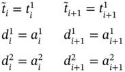
If both α1 < α and α3 > α are true (Figure 5.5b), then regardless of the value of α2, the data synchronization can be simplified to (5.148).
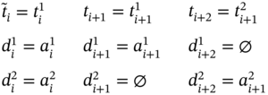
If both α1 > α and α2 < α are true (Figure 5.5c), then regardless of the value of α3, the data synchronization can be simplified to (5.149).
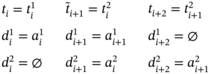
If either α1 > α > α2 > α3 or both α1 > α > α3 and α2 > α (Figure 5.5d) is true, the data synchronization can be simplified to (5.150).
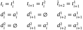
Thus, fuzzy synchronization allows us to simplify synchronization of data values measured at neighboring moments of time when the time difference is small enough that we can neglect this difference. We considered ![]() as the degree of closeness between time moments
as the degree of closeness between time moments ![]() and
and ![]() but other relation degrees defined in can be employed depending on a specific condition of the data synchronization task.
but other relation degrees defined in can be employed depending on a specific condition of the data synchronization task.
When the data sequences have been synchronized, we can compose a multi‐image of the object of study and process this multi‐image (which is the complex representation of all information we know about this object) employing the logical operations, ordering operations, arithmetical operations, and relations, which are defined in ASA, according to a specific logic and by using specific methods of solving a given task related to the object of study.
5.7 Conclusion
Multimodal data can be obtained in a wide range of applications in industry, medicine, engineering, etc., as a result of measurement, computing, modeling, prediction, and other data processing. The majority of approaches consider multimodal data sequences as separate ones like temperature data sequence, pressure data sequence, etc. However, complex representation of all multimodal data sequences as a sole mathematical object can be conducive to more effective solving of tasks related to multimodal data analysis and processing. In this chapter, we presented the apparatus of ASA that enables such complex representation and processing of multimodal data in the form of aggregates and multi‐images.
Multi‐images data synchronization is an important task because it ensures correct interpretation of multimodal data and their correlation in terms of time. Multimodal data synchronization can be fulfilled by using relations defined in ASA. After synchronization, we obtain the multi‐image, which is a complete timewise data structure, ready for further complex data analysis in such tasks as data modeling, prediction, classification, clustering, and other tasks. Further data processing can be fulfilled by using a domain‐specific program language such as ASAMPL [20].
References
- 1 Dychka, I. and Sulema, Y. (2019). Ordering operations in algebraic system of aggregates for multi‐image data processing. Research Bulletin of the National Technical University of Ukraine “Kyiv Polytechnic Institute” 1: 15–23.
- 2 Dychka, I. and Sulema, Y. (2018). Logical operations in algebraic system of aggregates for multimodal data representation and processing. Research Bulletin of the National Technical University of Ukraine “Kyiv Polytechnic Institute” 6: 44–52.
- 3 Maltsev, A.I. (1970). Algebraic Systems. Nauka.
- 4 Fraenkel, A.A., Bar‐Hillel, Y., Levy, A. et al. (1973). Foundations of Set Theory. Elsevier.
- 5 Kulik, B.A., Zuenko, A.A., and Fridman, A.Y. (2010). Algebraic Approach to Intellectual Processing of Data and Knowledge. Izdatelstvo Politekhnicheskogo Universiteta.
- 6 Petrovsky, A.B. (2003). Space of Sets and Multi‐sets. Editorial URSS.
- 7 Allen, J.F. (1983). Maintaining knowledge about temporal intervals. Communications of the ACM 26: 832–843. https://doi.org/10.1145/182.358434.
- 8 Allen, J.F. and Hayes, P.J. (1989). Moments and points in an interval‐based temporal logic. Computational Intelligence 5 (3): 225–238. https://doi.org/10.1111/j.1467-8640.1989.tb00329.x.
- 9 Nebel, B. and Bürckert, H.‐J. (1995). Reasoning about temporal relations: a maximal tractable subclass of Allen's interval algebra. Journal of the ACM 42 (1): 43–66.
- 10 Allen, J.F. and Ferguson, G. (1997). Actions and events in interval temporal logic. In: Spatial and Temporal Reasoning, 205–245. Springer https://doi.org/10.1007/978-0-585-28322-7_7.
- 11 Schockaert, S., De Cock, M., and Kerre, E. (2010). Reasoning About Fuzzy Temporal and Spatial Information from the Web, Intelligent Information Systems, vol. 3. World Scientific.
- 12 Bozzelli, L. et al. (2016). Interval vs. point temporal logic model checking: an expressiveness comparison. Proceedings of the 36th IARCS Annual Conference on Foundations of Software Technology and Theoretical Computer Science (FSTTCS 2016), Chennai, India (13–15 December 2016). Chennai: Chennai Mathematical Institute.
- 13 Grüninger, M. and Li, Z. (2017). The time ontology of Allen's interval algebra. Proceedings of 24th International Symposium on Temporal Representation and Reasoning (TIME 2017), Article No. 16, 16–18 October 2017, Mons, Belgium. LIPICS Schloss Dagstuhl – Leibniz‐Zentrum für Informatik GmbH, Dagstuhl Publishing, Saarbrücken/Wadern,Germany.
- 14 Guesgen, H.W., Hertzberg, J. and Philpott, A. (1994). Towards implementing fuzzy Allen relations. Proceedings of the ECAI‐94 Workshop on Spatial and Temporal Reasoning. August 8–12 Amsterdam, The Netherlands.
- 15 Bodenhofer, U. A new approach to fuzzy orderings. Tatra Mountains Mathematical Publications 16: 21–29.
- 16 Badaloni, S. and Giacomin, M. (2000). A fuzzy extension of Allen's interval algebra. Lecture Notes in Artificial Intelligence 1792: 155–165.
- 17 Dubois, D., Hadj Ali, A., and Prade, H. (2003). Fuzziness and uncertainty intemporal reasoning. Journal of Universal Computer Science 9: 1168–1194.
- 18 Schockaert, S., De Cock, M., and Kerre, E. (2008). Fuzzifying Allen's temporal interval relations. IEEE Transactions on Fuzzy Systems 16 (2): 517–533.
- 19 Bandler, W. and Kohout, L.J. (1980). Fuzzy relational products as a tool for analysis and synthesis of the behaviour of complex natural and artificial systems. In: Fuzzy Sets: Theory and Application to Policy Analysis and Information Systems (eds. S.K. Wang and P.P. Chang), 341–367. New York: Plenum.
- 20 Sulema, Y. (2018). ASAMPL: programming language for mulsemedia data processing based on algebraic system of aggregates. In: Interactive Mobile Communication Technologies and Learning. IMCL 2017, Advances in Intelligent Systems and Computing, vol. 725, 431–442. Springer https://doi.org/10.1007/978-3-319-75175-7_43.