6
Nonprobabilistic Analysis of Thermal and Chemical Diffusion Problems with Uncertain Bounded Parameters
Sukanta Nayak1, Tharasi Dilleswar Rao2, and Snehashish Chakraverty2
1Department of Mathematics, Amrita School of Engineering, Amrita Vishwa Vidyapeetham, Coimbatore, Tamil Nadu, 641112, India
2Department of Mathematics, National Institute of Technology Rourkela, Rourkela, Odisha, 769008, India
6.1 Introduction
Diffusion plays a major role in the field of thermal and chemical engineering. It may arise in a wide range of problems, viz., heat transfer, fluid flow, and chemical diffusion. These problems are governed by various linear and nonlinear differential equations. The problem with involved parameters, coefficients, and initial and boundary conditions greatly affects the solution of differential equations. In addition, the parameters used in the modeled physical problem are not crisp (or exact) because of the mechanical defect, experimental and measurement error, etc. In this context, the problem has to be defined with uncertain bounded parameters, which make it challenging to investigate. However, the uncertainties are handled by various authors using probability density functions or statistical methods, but these methods need plenty of data and also may not consider the vague or imprecise parameters. Accordingly, one may use interval and/or fuzzy computation in the analysis of the problems.
As such, this chapter comprises interval and/or fuzzy uncertainties along with well‐known numerical methods, viz., finite element and explicit finite difference methods (EFDMs) to investigate heat and gas diffusion problems. The interval and/or fuzzy finite element formulation for tapered fin and finite difference formulation for radon diffusion mechanism in uncertain environment are discussed in details.
6.2 Preliminaries
6.2.1 Interval Arithmetic
As the operating boundary conditions and involved parameters of the system are uncertain in nature, we may take such values as interval/fuzzy numbers. Initially, if the interval values are considered, then the arithmetic rules may be written as [1]
where ![]() and
and ![]() are the left and right values of the interval, respectively. For the same interval, mid value is
are the left and right values of the interval, respectively. For the same interval, mid value is ![]() and width
and width ![]() .
.
The traditional interval arithmetic for two arbitrary intervals [![]() ] and [
] and [![]() ] is defined as follows.
] is defined as follows.
Addition:
Subtraction:
Multiplication:
Division:
Because of the complexity of the traditional interval arithmetic, the same can be modified into the following parametric form [2].
Consider ![]() be an arbitrary interval, then
be an arbitrary interval, then ![]() can be written as
can be written as
where w is the width of the interval.
If all the values of the interval are in R+ or R−, then the arithmetic rules [3] may be written as
In spite of the complex representation, the beauty of this arithmetic is that for computational purpose, the one parametric representation is quite handy to use. In addition to this, the above form of the interval arithmetic has great utility over the traditional interval arithmetic. Using the above transformation, the interval values are transformed into crisp form and then mathematical limit is operated. The generalized versions of transformed crisp values may easily be handled. This arithmetic may be extended for fuzzy numbers, which is described in the succeeding paragraph.
6.2.2 Fuzzy Number and Fuzzy Arithmetic
A fuzzy number is defined as the normalized convex fuzzy set ![]() , which is piecewise continuous. An arbitrary fuzzy number
, which is piecewise continuous. An arbitrary fuzzy number ![]() is said to be triangular fuzzy number (TFN) when the membership function is given by
is said to be triangular fuzzy number (TFN) when the membership function is given by

The fuzzy numbers may be represented as an ordered pair form ![]() , 0 ≤ α ≤ 1, where
, 0 ≤ α ≤ 1, where ![]() and
and ![]() are left and right monotonic increasing and decreasing functions over [0, 1], respectively. The TFN
are left and right monotonic increasing and decreasing functions over [0, 1], respectively. The TFN ![]() may be transformed into interval form by using α−cut as follows (Figure 6.1).
may be transformed into interval form by using α−cut as follows (Figure 6.1).
![Geometry of a triangular fuzzy number represented as an ordered pair form depicted as
left and right monotonic increasing and decreasing functions over [0, 1].](https://imgdetail.ebookreading.net/202109/3/9781119585503/9781119585503__9781119585503__files__images__c06f001.jpg)
Figure 6.1 Triangular fuzzy number (TFN).
Let us consider two fuzzy numbers ![]() and
and ![]() and a scalar k then
and a scalar k then
- (a) x = y if and only if
 and
and  .
. - (b)
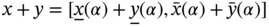 .
. - (c)
Combining both the fuzzy number and interval arithmetic, we may represent the fuzzy arithmetic as defined below [4,5].


where ![]() .
.
Here, the uncertain parameters are handled by using fuzzy values in place of classical (crisp) values. Therefore, we may combine the proposed fuzzy arithmetic and finite element method to develop fuzzy finite element method (FFEM) and the same can be used to solve various problems of engineering and science.
6.2.3 Parametric Representation of Fuzzy Number
The parametric approach is used to transform the interval‐based system of equations into crisp form [6,7]. As such, the interval ![]() may be transformed into crisp form as
may be transformed into crisp form as ![]() , where 0 ≤ β ≤ 1, it can also be written as
, where 0 ≤ β ≤ 1, it can also be written as
In order to obtain the lower and upper bounds of the solution in parametric form, we may substitute β = 0 and 1, respectively. Similar concept may be used for the multivariable uncertainty.
Table 6.1 Finite difference schemes for PDEs.
| Schemes | Derivative approximation of c(x, t) | |
| Forward | Derivatives with respect to x | Derivatives with respect to y |
 |
 | |
| Center | ||
 |
 | |
| Backward | ||
 |
 | |
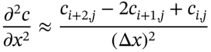
6.2.4 Finite Difference Schemes for PDEs
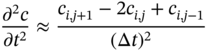
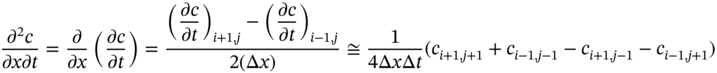
The numerical solutions of differential equations based on finite difference provide us with the values at discrete grid points in the domain of x − t plane. The spacing of the grid points in the x and t‐directions are assumed to be uniform as Δx and Δt. It is not necessary that Δx and Δy be uniform or equal to each other always. The grid points in the x‐direction are represented by index i and similarly j in the t direction. As such, the difference schemes for partial differential equations (PDEs) [8] are presented in Table 6.1.
To evaluate the derivative term ![]() , let us write the x‐direction as a central difference of t‐derivatives, and further, we make use of central difference to find out the y‐derivatives. Thus, we obtain
, let us write the x‐direction as a central difference of t‐derivatives, and further, we make use of central difference to find out the y‐derivatives. Thus, we obtain
Similarly, other difference schemes may also be written.
6.3 Finite Element Formulation for Tapered Fin
Let us consider a tapered fin with plane surfaces on the top and bottom. The fin also loses heat to the ambient via the tip. The thickness of the fin varies linearly from d1 at the base to d2 at the tip. The width b remains constant throughout the fin and L is the length.
Here, a typical element e1 is having nodes i and j, respectively, as shown in Figure 6.2. Then, the corresponding area (Ai and Aj) and perimeter (Pi and Pj) for nodes i and j, respectively, are (Figures 6.3 and 6.4)
The shape functions for each element are ![]() and
and ![]() , and the area of the fin varies linearly. Therefore, the area A of tapered fin may be expressed as follows.
, and the area of the fin varies linearly. Therefore, the area A of tapered fin may be expressed as follows.
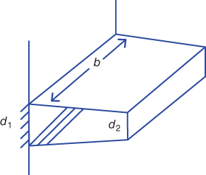
Figure 6.2 Model diagram of tapered fin.
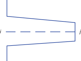
Figure 6.3 Tapered fin having two nodes.
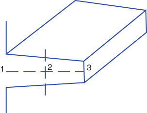
Figure 6.4 Two‐element discretization of tapered fin.
Similarly, perimeter P of tapered fin may be written as
The stiffness matrix for the corresponding tapered fin is [9]
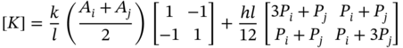
and the force vector is [9]

where G is the heat source per unit volume, q is the heat flux, h is the heat transfer coefficient, k is the thermal conductivity, Ta is the ambient temperature, and l is the length of each element. Here, in Eq. (6.21), the last term is valid only for the element at the end face with area A. For all other elements, the last term of Eq. (6.21) is zero.
Next considering the above finite element formulation of tapered fin, we have taken a numerical example of the same and obtained the corresponding results under uncertain environment.
Corresponding nodal temperatures for different numbers of discretization have been presented graphically in Figure 6.5.
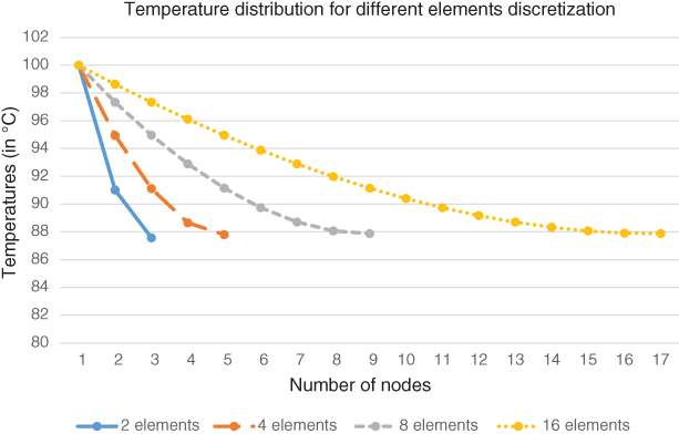
Figure 6.5 Nodal temperatures of tapered fin (crisp values).
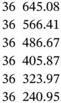
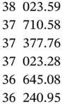
Now, considering the imprecise values as fuzzy, mentioned above, we get a series of nodal temperatures depending on the value of α. When the value of α becomes 1 (that is crisp), we get the series of nodal temperatures that are presented in Table 6.3. Similarly, when the value of α is zero, then the obtained results are mentioned in Table 6.4. It is worth mentioning that the value of α = 0 gives the interval results.
Next, as described in the introduction, numerical modeling of a chemical diffusion problem, viz., radon diffusion mechanism, in an uncertain scenario is investigated.
6.4 Radon Diffusion and Its Mechanism
Chemically, radon is a radioactive inert gas, which is formed by decay of 226Ra. It has been used as a trace gas in terrestrial, hydrogeological, and atmospheric studies. Radon is usually found in igneous rocks, soils, and groundwater, and inhalation of radon causes lung cancer [10,11]. Radon problem is a major concern in cold climate country. As such, measuring radon concentration levels in homes, mines, etc., with accuracy is an important task. Many researchers are working on various types of radon transport mechanisms. The transportation phenomena of radon in soil pore are mainly governed by two physical processes, namely, diffusion and advection. As such, different models have been developed based on these transport processes to study the anomalous behavior of soil radon in geothermal fields [12–14]. These models have been employed to estimate process‐driven parameters, viz., diffusion coefficient, carrier gas velocity from the measured data of soil radon. Estimation of these parameters may deviate significantly from the true values, if the uncertainty associated with the various input parameters of the models are not taken into consideration. Radon is also monitored as an earthquake precursor from decades along with the various other precursors [15,16]. However, prediction of the earthquake based on these precursors is still elusive. One of the main reasons for this is the uncertainty involved in the estimated values of the physical factors [17]. Therefore, modeling radon diffusion with uncertainty parameters is a challenging task [18,19]. In view of this, the targeted chapter investigates the numerical modeling, viz., EFDM to radon transport mechanism in an uncertain scenario.
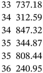
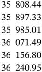
Table 6.4 Nodal temperatures of tapered fin (triangular fuzzy values).
| Elements | ||||||||
| 2 Elements | 4 Elements | 8 Elements | 16 Elements | |||||
| Left | Right | Left | Right | Left | Right | Left | Right | |
| T1 | 100 | 100 | 100 | 100 | 100 | 100 | 100 | 100 |
| T2 | 90.627 713 674 689 574 | 91.387 616 322 613 610 | 94.725 068 827 360 559 | 95.149 122 148 100 105 | 97.216 187 977 239 898 | 97.440 024 774 565 089 | 98.569 699 272 960 946 | 98.684 215 890 087 131 |
| T3 | 87.025 484 917 636 106 | 88.117 531 760 904 640 | 90.733 589 214 346 651 | 91.485 605 478 498 215 | 94.742 936 571 523 344 | 95.167 304 843 400 885 | 97.216 139 545 763 795 | 97.439 393 041 154 545 |
| T4 | 88.161 485 570 865 807 | 89.136 194 931 358 446 | 92.589 700 289 305 100 | 93.190 698 105 106 108 | 95.940 138 038 821 786 | 96.266 299 297 954 276 | ||
| T5 | 87.263 982 393 115 398 | 88.338 409 812 090 745 | 90.770 483 576 744 653 | 91.523 287 871 460 539 | 94.742 742 990 447 283 | 95.165 916 919 032 966 | ||
| T6 | 89.304 962 311 577 796 | 90.183 425 403 919 415 | 93.625 257 377 692 165 | 94.139 464 620 269 152 | ||||
| T7 | 88.220 023 585 389 711 | 89.196 161 218 768 083 | 92.589 266 407 343 786 | 93.188 423 120 981 795 | ||||
| T8 | 87.547 982 901 173 384 | 88.590 237 946 663 947 | 91.636 273 578 892 556 | 92.314 060 973 581 107 | ||||
| T9 | 87.341 103 368 466 506 | 88.415 517 289 493 224 | 90.768 912 809 597 111 | 91.518 964 462 502 808 | ||||
| T10 | 89.989 828 568 346 979 | 90.805 597 326 950 732 | ||||||
| T11 | 89.302 111 572 323 909 | 90.176 837 659 239 126 | ||||||
| T12 | 88.709 359 326 651 438 | 89.636 034 146 552 092 | ||||||
| T13 | 88.215747936824826 | 89.187072784234260 | ||||||
| T14 | 87.826 117 730 632 674 | 88.834 456 417 046 994 | ||||||
| T15 | 87.546 075 912 767 620 | 88.583 400 102 524 678 | ||||||
| T16 | 87.382 120 381 198 320 | 88.439 946 132 058 282 | ||||||
| T17 | 87.341 790 041 397 388 | 88.411 103 666 579 493 | ||||||
Corresponding nodal temperatures of Table 6.4 for different numbers of discretization with fuzzy parameters are also shown in Figure 6.6.
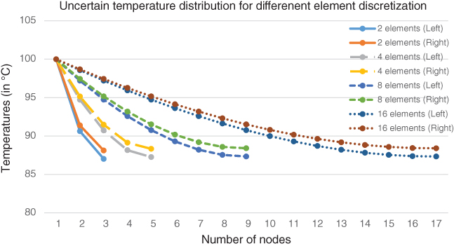
Figure 6.6 Nodal temperatures of tapered fin (left and right values).
Radon (Rn) is a radioactive inert gas that can be found in various mediums, viz., soil, water, air, etc., and it is subject to radioactive decay (Rn220and Rn219), which can cause radiation exposure problems. The spatial difference of radon concentration that exists between the surface (x = 0) and the underground induces a diffusive radon flow toward the surface. As such, the governing differential equations of radon flux density (J) and diffusion equation [13,14] are given as
where λ = 2.1 × 10⁻⁶s−1 (decay constant) and D = diffusion coefficient.
In general, diffusion of radon transforms from higher concentration region to lower concentration region with an initial radon concentration (c0) and radon uncertain flux density through the soil is zero before the diffusion starts (t = 0). Radon flux density increases with time; hence, the initial and boundary conditions for radon diffusion are as follows:

6.5 Radon Diffusion Mechanism with TFN Parameters
As discussed, the estimation of process‐driven parameters, viz., diffusion coefficient (D) and initial concentration (c0), from the measured data of soil radon may deviate significantly from the true values. Therefore, by considering D and c0 as uncertain parameters, we can represent radon diffusion equation as
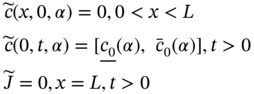
subject to uncertain boundary conditions

Here, the involved uncertain parameters ![]() and
and ![]() are considered as TFNs. As such, α− cut is used to transform the fuzzy‐based parameters to interval form as follows:
are considered as TFNs. As such, α− cut is used to transform the fuzzy‐based parameters to interval form as follows:

Accordingly, by using α− cut in the uncertain diffusion equation (Eq. (6.24)), one can transform into interval form as

subject to interval form initial and boundary conditions
Now, the interval form of Eq. (6.26) can be transformed into crisp form by using the parametric concept as
subject to initial and boundary conditions
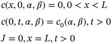
where

The next Section 6.5.1 presents numerical modeling of the above‐described uncertain radon diffusion problem by using EFDM.
6.5.1 EFDM to Radon Diffusion Mechanism with TFN Parameters
The central difference scheme is used to represent the term ![]() and a forward difference scheme for the term
and a forward difference scheme for the term ![]() in Eq. (6.27) to obtain numerical scheme as
in Eq. (6.27) to obtain numerical scheme as
subject to initial and boundary conditions


Figure 6.7 Crisp numerical solution of Eq. (6.24) by EFDM at different times (t) and α = 1.

Figure 6.8 Fuzzy numerical solution of Eq. (6.24) by EFDM at different times (t) and α, β.
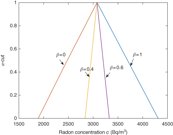
Figure 6.9 Radon concentration at c(4,500s, α, β).
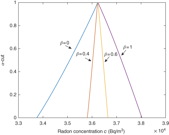
Figure 6.10 Radon concentration at c(4,12 000s, α, β).
where
![]() and b(α, β) = (1 − 2a(α, β) − λΔt).
and b(α, β) = (1 − 2a(α, β) − λΔt).
Here, indices i and j represent the discrete positions and times determined by step lengths Δx and Δt for the coordinates x and t, respectively. By varying the controlling parameters α, β ∈ [0, 1], one may handle the involved uncertainty of the considered model (Eq. (6.24)).
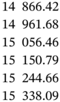
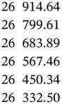
Table 6.5 : Radon concentration c(4, t, α, β) of Eq. (6.24) by EFDM.
| β | t−level | c((4, t, α, β)) | |||
| t = 500 seconds | t = 2000 seconds | t = 5000 seconds | t = 12 000 seconds | ||
 |
 |
 |
 | ||
 |
 |
 |
 | ||
 |
 |
 |
 | ||
 |
 |
 |
 | ||
As discussed in the above Section 6.5, α and β are the controlling parameters to handle the involved uncertainty of the considered model Eq. (6.24). As such, one can analyze the behavior or validation of the considered fuzzy radon model by using α and β. Accordingly, some of the outcomes are included and discussed here. Figure 6.7 depicts the center/crisp radon behavior for different times (t) and controlling parameter taken as α = 1. In addition, Figure 6.8 depicts the fuzzy numerical solution (lower, center, and upper) radon concentrations at different t by choosing (α, β = 0) for lower, α = 1 for center, and (α = 0, β = 1) to get upper concentration. By this modeling, one can estimate a fuzzy band at every t to investigate the behavior of radon gas.
Further, the involved imprecise parameters of the considered model are taken as TFNs. Therefore, the radon concentration is presented at different times (t) and also for different depths. Accordingly, Figure 6.9 characterizes the radon concentration for all α = 0.1 : 0.1 : 1 at a fixed depth (x = 4 cm) and time (t = 500 seconds). Similarly, the radon concentration for all α = 0.1 : 0.1 : 1 at a fixed depth (x = 4 cm) and time (t = 12 000 seconds) is also illustrated in Figure 6.10. Accordingly, by using the often values of the controlling parameters α, β ∈ [0, 1] with the depth (x) and time (t), one can investigate the behavior of radon concentration. The radon concentrations of the considered model (Eq. (6.24)) at different t and fixed depth x = 4 cm for some α, β ∈ [0, 1] are presented in Table 6.5. From this, one can observe an incremental growth in radon concentration with respect to the increment in t.
6.6 Conclusion
In this chapter, two different alternate approaches have been discussed to handle heat and chemical diffusion problems under an uncertain environment. Especially, the involved parameters, boundary conditions, and initial inputs are carried as uncertain, and accordingly, the uncertain governing differential equations have been investigated. The obtained results give good agreement with special cases, as well as the uncertain spectrum of the obtained solutions is easily illustrated in the given tables and figures. The above study shows that the discussed methods are not limited to the mentioned problems but may be useful to other diffusion and structure problems.
References
- 1 Moore, R.E., Baker Kearfott, R., and Cloud, M.J. (2009). Introduction to Interval Analysis. SIAM.
- 2 Nayak, S. and Chakraverty, S. (2013). Non‐probabilistic approach to investigate uncertain conjugate heat transfer in an imprecisely defined plate. International Journal of Heat and Mass Transfer 67: 445–454.
- 3 Nayak, S. and Chakraverty, S. (2015). Fuzzy finite element analysis of multigroup neutron diffusion equation with imprecise parameters. International Journal of Nuclear Energy Science and Technology 9 (1): 1–22.
- 4 Nayak, S. and Chakraverty, S. (2015). Numerical solution of uncertain neutron diffusion equation for imprecisely defined homogeneous triangular bare reactor. Sadhana 40: 2095–2109.
- 5 Nayak, S. and Chakraverty, S. (2018). Non‐probabilistic solution of moving plate problem with uncertain parameters. Journal of Fuzzy Set Valued Analysis 2: 49–59.
- 6 Behera, D. and Chakraverty, S. (2015). New approach to solve fully fuzzy system of linear equations using single and double parametric form of fuzzy numbers. Sadhana 40 (1): 35–49.
- 7 Tapaswini, S. and Chakraverty, S. (2013). Numerical solution of n‐th order fuzzy linear differential equations by homotopy perturbation method. International Journal of Computer Applications 64 (6): 5–10.
- 8 Chakraverty, S., Mahato, N., Karunakar, P., and Rao, T.D. (2019). Advanced Numerical and Semi‐Analytical Methods for Differential Equations. Wiley.
- 9 Nayak, S., Chakraverty, S., and Datta, D. (2014). Uncertain spectrum of temperatures in a non‐homogeneous fin under imprecisely defined conduction‐convection system. Journal of Uncertain Systems 8 (2): 123–135.
- 10 Nazaroff, W.W. (1992). Radon transport from soil to air. Reviews of Geophysics 30 (2): 137–160.
- 11 Schery, S.D., Holford, D.J., Wilson, J.L., and Phillips, F.M. (1988). The flow and diffusion of radon isotopes in fractured porous media Part 2, Semi infinite media. Radiation Protection Dosimetry 24 (1–4): 191–197.
- 12 Kozak, J.A., Reeves, H.W., and Lewis, B.A. (2003). Modeling radium and radon transport through soil and vegetation. Journal of Contaminant Hydrology 66 (3): 179–200.
- 13 Savović, S., Djordjevich, A., Peter, W.T., and Nikezić, D. (2011). Explicit finite difference solution of the diffusion equation describing the flow of radon through soil. Applied Radiation and Isotopes 69 (1): 237–240.
- 14 Kohl, T., Medici, F., and Rybach, L. (1994). Numerical simulation of radon transport from subsurface to buildings. Journal of Applied Geophysics 31 (1): 145–152.
- 15 Planinić, J., Radolić, V., and Vuković, B. (2004). Radon as an earthquake precursor. Nuclear Instruments and Methods in Physics Research Section A: Accelerators, Spectrometers, Detectors and Associated Equipment 530 (3): 568–574.
- 16 Fleischer, R.L. (1997). Radon and earthquake prediction. In: Radon Measurements by Etched Track Detectors: Applications in Radiation Protection, Earth Sciences and the Environment (eds. A. Durrani Saeed and I. Radomir), 285. World Scientific.
- 17 Chakraverty, S., Sahoo, B.K., Rao, T.D. et al. (2018). Modelling uncertainties in the diffusion‐advection equation for radon transport in soil using interval arithmetic. Journal of Environmental Radioactivity 182: 165–171.
- 18 Rao, T.D. and Chakraverty, S. (2017). Modeling radon diffusion equation in soil pore matrix by using uncertainty based orthogonal polynomials in Galerkin's method. Coupled Systems Mechanics 6 (4): 487–499.
- 19 Rao, T.D. and Chakraverty, S. (2018). Modeling radon diffusion equation by using fuzzy polynomials in Galerkin's method. In: Recent Advances in Applications of Computational and Fuzzy Mathematics, 75–93. Singapore: Springer.