1
Connectionist Learning Models for Application Problems Involving Differential and Integral Equations
Susmita Mall, Sumit Kumar Jeswal, and Snehashish Chakraverty
Department of Mathematics, National Institute of Technology Rourkela, Rourkela, Odisha, 769008, India
1.1 Introduction
1.1.1 Artificial Neural Network
Artificial intelligence (AI) also coined as machine intelligence is the concept and development of intelligent machines that work and react like humans. In the twentieth century, AI has a great impact starting from human life to various industries. Researchers from various parts of the world are developing new methodologies based on AI so as to make human life more comfortable. AI has different research areas such as artificial neural network (ANN), genetic algorithm (GA), support vector machine (SVM), fuzzy concept, etc.
In 1943, McCulloh and Pitts [1] designed a computational model for neural network based on mathematical concepts. The concept of perceptron has been proposed by Rosenblatt [2]. In the year 1975, Werbos [3] introduced the well‐known concept of backpropagation algorithm. After the creation of backpropagation algorithm, different researchers explored the various aspects of neural network.
The concept of ANN inspires from the biological neural systems. Neural network consists of a number of identical units known as artificial neurons. Mainly, neural network comprises three layers, viz., input, hidden, and output. Each neuron in the nth layer has been interconnected with the neurons of the (n + 1)th layer by some signal. Each connection has been assigned with weight. The output has been calculated after multiplying each input with its corresponding weight. Further, the output passes through an activation function to get the desired output.
ANN has various applications in the field of engineering and science such as image processing, weather forecasting, function approximation, voice recognition, medical diagnosis, robotics, signal processing, etc.
1.1.2 Types of Neural Networks
There are various types of neural network models, but commonly used models have been discussed further.
- Feedforward neural network: In feedforward network, the connection between the neurons does not form a cycle. In this case, the information passes through in one direction.
- Single‐layer perceptron: It is a simple form of feedforward network without having hidden layers, viz., function link neural network (FLNN).
- Multilayer perceptron: Multilayer perceptron is feedforward network, which comprises of three layers, viz., input, hidden, and output.
- Convolutional neural network (CNN): CNN is a class of deep neural networks that is mostly used in analyzing visual imagery.
- Feedback or recurrent neural network: In feedback neural network, the different connections between the neurons form a directed cycle. In this case, the information flow is bidirectional.
The general model of an ANN has been depicted in Figure 1.1.
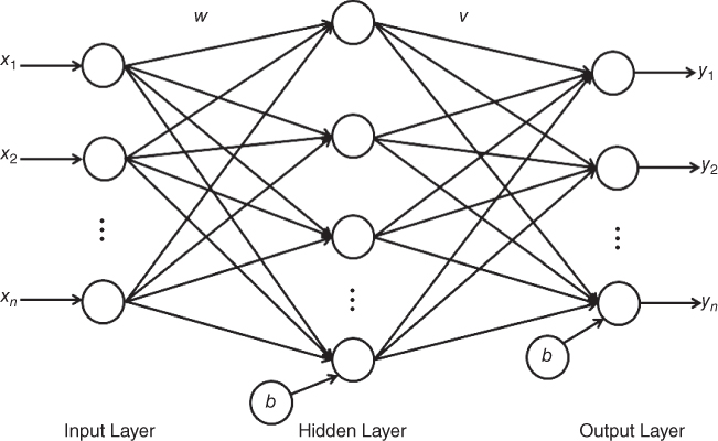
Figure 1.1 General model of ANN.
1.1.3 Learning in Neural Network
There are mainly three types of learning, viz., supervised or learning with a teacher, unsupervised or learning without a teacher, and reinforcement learning. In the supervised case, the desired output of the ANN model is known, but on the other hand, the desired output is unknown in the case of unsupervised learning. In reinforcement learning, the ANN model learns its behavior based on the feedback from the environment. Various learning rules have been developed to train or update the weights. Some of them are mentioned below.
- (a) Hebbian learning rule
- (b) Perceptron learning rule
- (c) Delta learning rule or backpropagation learning rule
- (d) Out star learning rule
- (e) Correlation learning rule
1.1.4 Activation Function
An output node receives a number of input signals, depending on the intensity of input signals, we summed these input signals and pass them through some function known as activation function. Depending on the input signals, it generates an output and accordingly further actions have been performed. There are different types of activation functions from which some of them are listed below.
- Identity function
- Bipolar step function
- Binary step function
- Sigmoidal function
- Unipolar sigmoidal function
- Bipolar sigmoidal function
- Tangent hyperbolic function
- Rectified linear unit (ReLU)
Although we have mentioned a number of activation functions, but for the sake of completeness, we have just discussed about sigmoidal function below.
1.1.4.1 Sigmoidal Function
Sigmoidal function is a type of mathematical function that takes the form of an S‐shaped curve or a sigmoid curve.
There are two types of sigmoidal functions depending on their range.
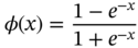
- Unipolar sigmoidal function: The unipolar sigmoidal function can be defined as

In this case, the range of the output lies within the interval [0, 1].
- Bipolar sigmoidal function: The bipolar sigmoidal function can be formulated as
The output range for bipolar case lies between [−1, 1]. Figure 1.2 represents the bipolar sigmoidal function.
1.1.5 Advantages of Neural Network
- (a) The ANN model works with incomplete or partial information.
- (b) Information processing has been done in a parallel manner.
- (c) An ANN architecture learns and need not to be programmed.
- (d) It can handle large amount of data.
- (e) It is less sensitive to noise.
1.1.6 Functional Link Artificial Neural Network (FLANN)
Functional Link Artificial Neural Network (FLANN) is a class of higher order single‐layer ANN models. FLANN model is a flat network without an existence of a hidden layer, which makes the training algorithm of the network less complicated. The single‐layer FLANN model is developed by Pao [4,5] for function approximation and pattern recognition with less computational cost and faster convergence rate. In FLANN, the hidden layer is replaced by a functional expansion block for artificial enhancement of the input patterns using linearly independent functions such as orthogonal polynomials, trigonometric polynomials, exponential polynomials, etc. Being a single‐layer model, its number of parameters is less than multilayer ANN. Thus, FLNN model has less computational complexity and higher convergence speed. In recent years, many researchers have commonly used various types of orthogonal polynomials, viz., Chebyshev, Legendre, Hermite, etc., as a basis of FLANN.
![Grid chart depicting a curve representing the bipolar sigmoidal function. The output range for bipolar case lies between [−1, 1].](https://imgdetail.ebookreading.net/202109/3/9781119585503/9781119585503__9781119585503__files__images__c01f002.jpg)
Figure 1.2 Sigmoidal function.
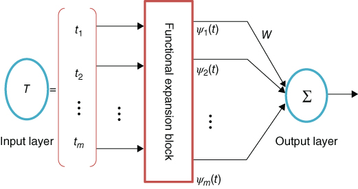
Figure 1.3 Structure of FLANN model.
As such, Chebyshev neural network model is widely used for handling various complicated problems, viz., function approximation [6], channel equalization [7], digital communication [8], solving nonlinear differential equations (DEs) [9,10], system identification [11,12], etc. Subsequently, Legendre neural network has been used for solving DEs [13], system identification [14], and for prediction of machinery noise [15]. Also, Hermite neural network is used for solving Van der Pol Duffing oscillator equations [16,17].
Figure 1.3 shows the structure of FLANN model, which consists of an input layer, a set of basis functions, a functional expansion block, and an output layer. The input layer contains T = [t1, t2, t3, …, tm] input vectors, a set of m basis functions {ψ1, ψ2, …, ψm} ∈ BM, and weight vectors W = [w1, w2, …, wm] from input to output layer associated with functional expansion block. The output of FLANN with the following input–output relationship may be written as
here, T ∈ Rm and ![]() denote the input and output vectors of FLANN, respectively, ψj(T) is the expanded input data with respect to basis functions, and wji stands for the weight associated with the jth output. The nonlinear differentiable functions, viz., sigmoid, tan hyperbolic, etc., are considered as an activation function λ(·) of single‐layer FLANN model.
denote the input and output vectors of FLANN, respectively, ψj(T) is the expanded input data with respect to basis functions, and wji stands for the weight associated with the jth output. The nonlinear differentiable functions, viz., sigmoid, tan hyperbolic, etc., are considered as an activation function λ(·) of single‐layer FLANN model.
1.1.7 Differential Equations (DEs)
Mathematical representation of scientific and engineering problem(s) is called a mathematical model. The corresponding equation for the system is generally given by differential equation (ordinary and partial), and it depends on the particular physical problem. As such, there exist various methods, namely, exact solution when the differential equations are simple, and numerical methods, viz., Runge–Kutta, predictor–corrector, finite difference, finite element when the differential equations are complex. Although these numerical methods provide good approximations to the solution, they require a discretization of the domain (via meshing), which may be challenging in two or higher dimensional problems.
In recent decade, many researchers have used ANN techniques for solving various types of ordinary differential equations (ODEs) [18–21] and partial differential equations (PDEs) [22–25]. ANN‐based approximate solutions of DEs are more advantageous than other traditional numerical methods. ANN method is general and can be applied to solve linear and nonlinear singular initial value problems. Computational complexity does not increase considerably with the increase in number of sampling points and dimension of the problem. Also, we may use ANN model as a black box to get numerical results at any arbitrary point in the domain after training of the model.
1.1.8 Integral Equation
Integral equations are defined as the equations where an unknown function appears under an integral sign. There are mainly two types of integral equations, viz., Fredholm and Volterra. ANN is a novel technique for handling integral equations. As such, some articles related to integral equations have been discussed. Golbabai and Seifollahi [26] proposed a novel methodology based on radial basis function network for solving linear second‐order integral equations of Fredholm and Volterra types. An radial basis function (RBF) network has been presented by Golbabai et al. [27] to find the solution of a system of nonlinear integral equations. Jafarian and Nia [28] introduced ANN architecture for solving second kind linear Fredholm integral systems. A novel ANN‐based model has been developed by Jafarian et al. [29] for solving a second kind linear Volterra integral equation system. S. Effati and Buzhabadi [30] proposed a feedforward neural network‐based methodology for solving Fredholm integral equations of second kind. Bernstein polynomial expansion method has been used by Jafarian et al. [31] for solving linear second kind Fredholm and Volterra integral equation systems. Kitamura and Qing [32] found the numerical solution of Fredholm integral equations of first kind using ANN. Asady et al. [33] constructed a feedforward ANN architecture to solve two‐dimensional Fredholm integral equations. Radial basis functions have been chosen to find an iterative solution for linear integral equations of second kind by Golbabai and Seifollahi [34]. Cichocki and Unbehauen [35] gave a neural network‐based method for solving a linear system of equations. A multilayer ANN architecture has been proposed by Jeswal and Chakraverty [36] for solving transcendental equation.
1.1.8.1 Fredholm Integral Equation of First Kind
The Fredholm equation of first kind can be defined as

where K is called kernel and φ and f are the unknown and known functions, respectively. The limits of integration are constants.
1.1.8.2 Fredholm Integral Equation of Second Kind
The Fredholm equation of second kind is
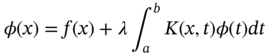
here, λ is an unknown parameter.
1.1.8.3 Volterra Integral Equation of First Kind
The Volterra integral equation of first kind is defined as

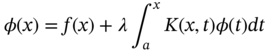
1.1.8.4 Volterra Integral Equation of Second Kind
The Volterra Integral equation of second kind may be written as
1.1.8.5 Linear Fredholm Integral Equation System of Second Kind
A system of linear Fredholm integral equations of second kind may be formulated as [28]
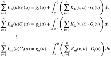
here, u, v ∈ [a, b] and L(u), K(v, u) are real functions. G(u) = [G1(u), G2(u), …, Gn(u)] is the solution set to be found.
1.2 Methodology for Differential Equations
1.2.1 FLANN‐Based General Formulation of Differential Equations
In this section, general formulation of differential equations using FLANN has been described. In particular, the formulations of ODEs are discussed here.
In general, differential equations (ordinary as well as partial) can be written as [18]
where F defines the structure of DEs, ∇ stands for differential operator, and y(t) is the solution of DEs. It may be noted that for ODEs ![]() and for PDEs
and for PDEs ![]() . Let yLg(t, p) denotes the trial solution of FLANN (Laguerre neural network, LgNN) with adjustable parameters p and then the above general differential equation changes to the form
. Let yLg(t, p) denotes the trial solution of FLANN (Laguerre neural network, LgNN) with adjustable parameters p and then the above general differential equation changes to the form
The trial solution yLg(t, p) satisfies the initial and boundary conditions and may be formulated as
where K(t) satisfies the boundary/initial conditions and contains no weight parameters. N(t, p) denotes the single output of FLANN with parameters p and input t. H(t, N(t, p)) makes no contribution to the initial or boundary conditions, but it is used in FLANN where weights are adjusted to minimize the error function.
The general form of corresponding error function for the ODE can be expressed as

We take some particular cases in Sections 1.2.1.1 and 1.2.1.2.
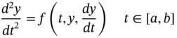
1.2.1.1 Second‐Order Initial Value Problem
Second‐order initial value problem may be written as

with initial conditions y(a) = C, ![]() .
.
The LgNN trial solution is formulated as
The error function is computed as follows

1.2.1.2 Second‐Order Boundary Value Problem
Next, let us consider a second‐order boundary value problem as
with boundary conditions y(a) = A, y(b) = B.
The LgNN trial solution for the above boundary value problem is
In this case, the error function is the same as Eq. (1.7).
1.2.2 Proposed Laguerre Neural Network (LgNN) for Differential Equations
Here, we have included architecture of LgNN, general formulation for DEs, and its learning algorithm with gradient computation of the ANN parameters with respect to its inputs.
1.2.2.1 Architecture of Single‐Layer LgNN Model
Structure of single‐layer LgNN model has been displayed in Figure 1.4. LgNN is one type of FLANN model based on Laguerre polynomials. LgNN consists of single‐input node, single‐output node, and functional expansion block of Laguerre orthogonal polynomials. The hidden layer is removed by transforming the input data to a higher dimensional space using Laguerre polynomials. Laguerre polynomials are the set of orthogonal polynomials obtained by solving Laguerre differential equation

Figure 1.4 Structure of single‐layer Laguerre neural network.
These are the first few Laguerre polynomials
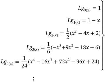
The higher order Laguerre polynomials may be generated by recursive formula
Here, we have considered that one input node has h number of data, i.e. t = (t1, t2, …, th)T. Then, the functional expansion block of input data is determined by using Laguerre polynomials as
In view of the above discussion, main advantages of the single‐layer LgNN model for solving differential equations may be given as follows:
- The total number of network parameters is less than that of traditional multilayer ANN.
- It is capable of fast learning and is computationally efficient.
- It is simple to implement.
- There are no hidden layers in between the input and output layers.
- The backpropagation algorithm is unsupervised.
- No other optimization technique is to be used.
1.2.2.2 Training Algorithm of Laguerre Neural Network (LgNN)
Backpropagation (BP) algorithm with unsupervised training has been applied here for handling differential equations. The idea of BP algorithm is to minimize the error function until the FLANN learned the training data. The gradient descent algorithm has been used for training and the network parameters (weights) are updated by taking negative gradient at each step (iteration). The training of the single‐layer LgNN model is to start with random weight vectors from input to output layer.
We have considered the nonlinear tangent hyperbolic (tanh) function, viz., ![]() , as the activation function.
, as the activation function.
The output of LgNN may be formulated as
where t is the input data, p stands for weights of LgNN, and s is the weighted sum of expanded input data. It is formulated as

where Lgk − 1(t) and wk with k = {1, 2, 3, …, m} are the expanded input and weight vector, respectively, of the LgNN model.
The weights are modified by taking negative gradient at each step of iteration
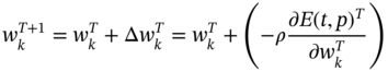
here, ρ is the learning parameter, T is the step of iteration, and E(t, p) denotes the error function of LgNN model.
1.2.2.3 Gradient Computation of LgNN
Derivatives of the network output with respect to the corresponding inputs are required for error computation. As such, derivative of N(t, p) with respect to t is

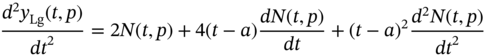
Similarly, the second derivative of N(t, p) can be computed as

After simplifying Eq. (1.18), we get

where wk denotes the weights of LgNN and ![]() are the first and second derivatives of Laguerre polynomials, respectively.
are the first and second derivatives of Laguerre polynomials, respectively.
Differentiate Eq. (1.6) with respect to t
Finally, the converged LgNN results may be used in Eqs. (1.6) and (1.9) to obtain the approximate results.
1.3 Methodology for Solving a System of Fredholm Integral Equations of Second Kind
While solving a system of Fredholm integral equations, it leads to a system of linear equations. Therefore, we have proposed an ANN‐based method for solving the system of linear equations.
A linear system of equations is written as
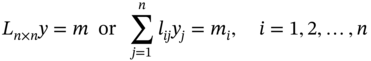
where L = [lij] is a n × n matrix, y = [y1, y2, …, yn]T is a n × 1 unknown vector, and m = [m1, m2, …, mn]T is a n × 1 known vector.
From Eq. (1.21), the vector ![]() and mi have been chosen as the input and target output of the ANN model, respectively. Further, y is the weights of the discussed ANN model, which can be shown in Figure 1.5.
and mi have been chosen as the input and target output of the ANN model, respectively. Further, y is the weights of the discussed ANN model, which can be shown in Figure 1.5.

Figure 1.5 ANN model for solving linear systems.
Taking the input, target output, and weights, training of the ANN model has been done until weight vector y matches the target output m.
The ANN output has been calculated as

where f is the activation function, which is chosen to be the identity function in this case.
The error term can be computed as
where ei = mi − zi.
The weights have been adjusted using the steepest descent algorithm as

and the updated weight matrix is given by
where η is the learning parameter and y(q) is the q‐th updated weight vector.
An algorithm for solving linear systems has been included in Section 1.3.1.
1.3.1 Algorithm
- Step 1: Choose the precision tolerance “tol,” learning rate η, random weights, q = 0 and E = 0;
- Step 2: Calculate
 , ei = mi − zi;
 - Step 3: The error term is given by

and weight updating formula is
where

If E < tol, then go to step 2, else go to step 4.
- Step 4: Print y.
1.4 Numerical Examples and Discussion
1.4.1 Differential Equations and Applications
In this section, a boundary value problem, a nonlinear Lane‐Emden equation, and an application problem of Duffing oscillator equation have been investigated to show the efficiency and powerfulness of the proposed method. In all cases, the feedforward neural network and unsupervised BP algorithm have been used for training. The initial weights from the input layer to the output layer are taken randomly.
1.4.2 Integral Equations
In this section, we have investigated three example problems of a system of Fredholm integral equations of second kind. The system of integral equations may be converted to a linear system using the trapezoidal rule. As such, a feedforward neural network model has been proposed for solving linear system.
1.5 Conclusion
As we know, most of the fundamental laws of nature may be formulated as differential equations. Numerous practical problems of mathematics, physics, engineering, economics, etc., can be modeled by ODEs and PDEs. In this chapter, the single‐layer FLANN, namely, LgNN model has been developed for solving ODEs. The accuracy of the proposed method has been examined by solving a boundary value problem, a second‐order singular Lane‐Emden equation, and an application problem of Duffing oscillator equation. In LgNN, the hidden layer is replaced by a functional expansion block of the input data by using Laguerre orthogonal polynomials. The LgNN computed results are shown in terms of tables and graphs.
Systems of Fredholm and Volterra equations are developing great interest for research in the field of science and engineering. In this chapter, an ANN‐based method for handling system of Fredholm equations of second kind has been investigated. The system of Fredholm equations has been transformed to a linear system using trapezoidal rule. As such, a single‐layer ANN architecture has been developed for solving the linear system. Comparison table between the exact and ANN solutions has been included. Further, convergence plots for solutions of different linear systems have been illustrated to show the efficacy of the proposed ANN algorithm.
References
- 1 McCulloh, W.S. and Pitts, W. (1943). A logical calculus of the ideas immanent in neural nets. Bulletin of Mathematical Biophysics 5 (4): 133–137.
- 2 Rosenblatt, F. (1958). The perceptron: a probalistic model for information storage and organization in the brain. Psychological Review 65 (6): 386–408.
- 3 Werbos, P.J. (1975). Beyond Regression: New Tools for Prediction and Analysis in the Behavioral Sciences. Harvard University.
- 4 Pao, Y.H. (1989). Adaptive Pattern Recognition and Neural Networks. Addison‐Wesley Longman Publishing Co., Inc.
- 5 Pao, Y.H. and Klaseen, M. (1990). The functional link net in structural pattern recognition. IEEE TENCON'90: 1990 IEEE Region 10 Conference on Computer and Communication Systems. Conference Proceedings, Hong Kong (24–27 September 1990). IEEE.
- 6 Lee, T.T. and Jeng, J.T. (1998). The Chebyshev‐polynomials‐based unified model neural networks for function approximation. IEEE Transactions on Systems, Man, and Cybernetics Part B: Cybernetics 28: 925–935.
- 7 Weng, W.D., Yang, C.S., and Lin, R.C. (2007). A channel equalizer using reduced decision feedback Chebyshev functional link artificial neural networks. Information Sciences 177: 2642–2654.
- 8 Patra, J.C., Juhola, M., and Meher, P.K. (2008). Intelligent sensors using computationally efficient Chebyshev neural networks. IET Science, Measurement and Technology 2: 68–75.
- 9 Mall, S. and Chakraverty, S. (2015). Numerical solution of nonlinear singular initial value problems of Emden–Fowler type using Chebyshev neural network method. Neurocomputing 149: 975–982.
- 10 Mall, S. and Chakraverty, S. (2014). Chebyshev neural network based model for solving Lane–Emden type equations. Applied Mathematics and Computation 247: 100–114.
- 11 Purwar, S., Kar, I.N., and Jha, A.N. (2007). Online system identification of complex systems using Chebyshev neural network. Applied Soft Computing 7: 364–372.
- 12 Patra, J.C. and Kot, A.C. (2002). Nonlinear dynamic system identification using Chebyshev functional link artificial neural network. IEEE Transactions on Systems, Man, and Cybernetics Part B: Cybernetics 32: 505–511.
- 13 Mall, S. and Chakraverty, S. (2016). Application of Legendre neural network for solving ordinary differential equations. Applied Soft Computing 43: 347–356.
- 14 Patra, J.C. and Bornand, C. (2010). Nonlinear dynamic system identification using Legendre neural network. The 2010 International Joint Conference on Neural Networks (IJCNN), Barcelona, Spain (18–23 July 2010). IEEE.
- 15 Nanda, S.K. and Tripathy, D.P. (2011). Application of functional link artificial neural network for prediction of machinery noise in opencast mines. Advances in Fuzzy Systems 2011: 1–11.
- 16 Mall, S. and Chakraverty, S. (2016). Hermite functional link neural network for solving the Van der Pol‐Duffing oscillator equation. Neural Computation 28 (8): 1574–1598.
- 17 Chakraverty, S. and Mall, S. (2017). Artificial Neural Networks for Engineers and Scientists: Solving Ordinary Differential Equations. CRC Press/Taylor & Francis Group.
- 18 Lagaris, I.E., Likas, A., and Fotiadis, D.I. (1998). Artificial neural networks for solving ordinary and partial differential equations. IEEE Transactions on Neural Networks 9: 987–1000.
- 19 Malek, A. and Beidokhti, R.S. (2006). Numerical solution for high order differential equations, using a hybrid neural network – optimization method. Applied Mathematics and Computation 183: 260–271.
- 20 Yazid, H.S., Pakdaman, M., and Modaghegh, H. (2011). Unsupervised kernel least mean square algorithm for solving ordinary differential equations. Neurocomputing 74: 2062–2071.
- 21 Selvaraju, N. and Abdul Samath, J. (2010). Solution of matrix Riccati differential equation for nonlinear singular system using neural networks. International Journal of Computer Applications 29: 48–54.
- 22 Shirvany, Y., Hayati, M., and Moradian, R. (2009). Multilayer perceptron neural networks with novel unsupervised training method for numerical solution of the partial differential equations. Applied Soft Computing 9: 20–29.
- 23 Aarts, L.P. and Van der Veer, P. (2001). Neural network method for solving partial differential equations. Neural Processing Letters 14: 261–271.
- 24 Hoda, S.A. and Nagla, H.A. (2011). Neural network methods for mixed boundary value problems. International Journal of Nonlinear Science 11: 312–316.
- 25 McFall, K. and Mahan, J.R. (2009). Artificial neural network for solution of boundary value problems with exact satisfaction of arbitrary boundary conditions. IEEE Transactions on Neural Networks 20: 1221–1233.
- 26 Golbabai, A. and Seifollahi, S. (2006). Numerical solution of the second kind integral equations using radial basis function networks. Applied Mathematics and Computation 174 (2): 877–883.
- 27 Golbabai, A., Mammadov, M., and Seifollahi, S. (2009). Solving a system of nonlinear integral equations by an RBF network. Computers & Mathematics with Applications 57 (10): 1651–1658.
- 28 Jafarian, A. and Nia, S.M. (2013). Utilizing feed‐back neural network approach for solving linear Fredholm integral equations system. Applied Mathematical Modelling 37 (7): 5027–5038.
- 29 Jafarian, A., Measoomy, S., and Abbasbandy, S. (2015). Artificial neural networks based modeling for solving Volterra integral equations system. Applied Soft Computing 27: 391–398.
- 30 Effati, S. and Buzhabadi, R. (2012). A neural network approach for solving Fredholm integral equations of the second kind. Neural Computing and Applications 21 (5): 843–852.
- 31 Jafarian, A., Nia, S.A.M., Golmankhaneh, A.K., and Baleanu, D. (2013). Numerical solution of linear integral equations system using the Bernstein collocation method. Advances in Difference Equations 2013 (1): 123.
- 32 Kitamura, S. and Qing, P. (1989). Neural network application to solve Fredholm integral equations of the first kind. In: Joint International Conference on Neural Networks, 589. IEEE.
- 33 Asady, B., Hakimzadegan, F., and Nazarlue, R. (2014). Utilizing artificial neural network approach for solving two‐dimensional integral equations. Mathematical Sciences 8 (1): 117.
- 34 Golbabai, A. and Seifollahi, S. (2006). An iterative solution for the second kind integral equations using radial basis functions. Applied Mathematics and Computation 181 (2): 903–907.
- 35 Cichocki, A. and Unbehauen, R. (1992). Neural networks for solving systems of linear equations and related problems. IEEE Transactions on Circuits and Systems I: Fundamental Theory and Applications 39 (2): 124–138.
- 36 Jeswal, S.K. and Chakraverty, S. (2018). Solving transcendental equation using artificial neural network. Applied Soft Computing 73: 562–571.
- 37 Ibraheem, K.I. and Khalaf, M.B. (2011). Shooting neural networks algorithm for solving boundary value problems in ODEs. Applications and Applied Mathematics 6: 187–200.
- 38 Lane, J.H. (1870). On the theoretical temperature of the sun under the hypothesis of a gaseous mass maintaining its volume by its internal heat and depending on the laws of gases known to terrestrial experiment. The American Journal of Science and Arts, 2nd series 4: 57–74.
- 39 Emden, R. (1907). Gaskugeln: Anwendungen der mechanischen Warmen‐theorie auf Kosmologie and meteorologische Probleme. Leipzig: Teubner.
- 40 Chowdhury, M.S.H. and Hashim, I. (2007). Solutions of a class of singular second order initial value problems by homotopy‐perturbation method. Physics Letters A 365: 439–447.
- 41 Vanani, S.K. and Aminataei, A. (2010). On the numerical solution of differential equations of Lane‐Emden type. Computers & Mathematics with Applications 59: 2815–2820.
- 42 Zhihong, Z. and Shaopu, Y. (2015). Application of van der Pol–Duffing oscillator in weak signal detection. Computers and Electrical Engineering 41: 1–8.
- 43 Jalilvand, A. and Fotoohabadi, H. (2011). The application of Duffing oscillator in weak signal detection. ECTI Transactions on Electrical Engineering, Electronics, and Communications 9: 1–6.