
Chapter 3. Computational transport processes for micromixers∗
Chapter Outline
3.1. Introduction74
3.2. Problem Description75
3.3. Mathematical Formulation75
3.4. Solution Procedure82
3.5. Verifications and Validations88
3.6. Examples92
3.6.1. Mixing in a micro-enclosure92
3.6.2. Mixing in a lid-driven microcavity92
3.6.3. Mixing in a straight microchannel96
3.6.4. Mixing in winding microchannels96
3.6.5. Mixing within a droplet flowing in a straight microchannel97
3.6.6. Mixing within a droplet flowing through a micro-U-bend100
3.6.7. Mixing in three thermocapillary merged droplets101
3.6.8. Mixing within a droplet driven by electroosmotic flow in an enclosure104
3.6.9. Mixing within a ferrofluid droplet107
3.7. Concluding Remarks110
References111
With a great variety of potential applications, transport processes in a micromixer are often rich in physics. Understanding these processes is crucial to the design of a good micromixer. As both the time and length scales involved are small, experimental investigations of these processes become increasingly challenging. Expensive high-resolution measurement equipment are required to provide data with time and length scales convincingly resolved. In view of this problem, theoretical investigations play an essential complementary role in the design of micromixers. Theoretical investigations provide useful detailed insights into the physics of the transport processes. It offers the ability to predict these transport processes.
3.1. Introduction
With a great variety of potential applications, transport processes in a micromixer are often rich in physics. Understanding these processes is crucial to the design of a good micromixer. As both the time and length scales involved are small, experimental investigations of these processes become increasingly challenging. Expensive high-resolution measurement equipment are required to provide data with time and length scales convincingly resolved. In view of this problem, theoretical investigations play an essential complementary role in the design of micromixers. Theoretical investigations provide useful detailed insights into the physics of the transport processes. It offers the ability to predict these transport processes.
∗This chapter is contributed by Yit Fatt Yap (Petroleum Institute, United Arab Emirates), Jing Liu (Nanyang Technological University, Singapore), and John Chee Kiong Chai (Petroleum Institute, United Arab Emirates).
Of particular interest in this chapter is the prediction of transport processes in micromixers. Generally, these processes involve the transport of physically and/or chemically distinct species. These processes can be affected by, among others, the flow, temperature, electric, and magnetic fields. These physical fields are often interrelated. As a result, the mixing process is governed by a system of strongly coupled partial differential equations (PDEs). These PDEs can be highly nonlinear. The geometries of the domain in which the solutions are sought for this system of PDEs are mostly irregular, in the sense that the boundary of the domain cannot be conveniently represented using an ordinary or even general curvilinear coordinate system. Attempting an analytical solution for this system of PDEs in irregular domains is mathematically very demanding. It is, therefore, not surprising that there are only a limited number of analytical solutions available, often at the cost of having assumptions that over-simplify the systems of PDEs. For such types of problems, a numerical solution is one of the most viable options leading to the subject of this chapter.
This chapter presents a general computational framework for the prediction of mixing process at the continuum level (see Chapter 2). The numerical engine for the framework is based on the finite volume method. This is the authors' biased personal choice after having worked on the finite volume method in recent years. Such a framework is equally applicable to other numerical engines based on the finite difference or the finite element method. This chapter focuses on the framework, for which solutions for the system of PDEs can be made, rather than on the various numerical approaches. Therefore, a comprehensive review of all the available literature related to various numerical approaches will not be attempted here. In the interest of providing a concise description of the computational framework implemented by the authors, it is possible that many significant papers might be omitted. Any such omissions are unintentional and do not imply any judgment as to the quality and usefulness of these works.
The remaining chapter is divided into five sections. A description of the problem is given in Section 3.2. In Section 3.3, the mathematical formulation of the problem is presented, including a discussion of an outline for incorporating various additional physics. The numerical solution procedure is given in Section 3.4. Section 3.5 is devoted to the verifications and validations of the solution procedures. Examples of mixing problems solved with the current framework are then presented and discussed in Section 3.6. Finally, the chapter concludes with a few remarks on the presented computational framework.
3.2. Problem Description
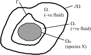
Let us consider a region Ω with boundary ∂Ω as shown in Figure 3.1. In the region Ω, there exists a fluid with a suspension of species X. Initially, species X is concentrated within the subregion ΩD. As time passes, driven by the underlying velocity field (convection) and concentration gradient of the species X (diffusion), species X spreads beyond ΩD. There can be a source/sink of the species X within Ω due to the formation/destruction of the species X, e.g., in chemical reactions. Besides, fluid flows across the boundary ∂Ω can bring in or take out species X. As an end effect, a mixing process of species X with the fluid occurs.

The mixing process described above involves transport of the species X and the fluid, and serves as the starting point of the computational framework for predicting mixing process in a micromixer. Additional physics involving temperature and electric or magnetic field on the mixing process can then be included into this framework.
3.3. Mathematical Formulation
3.3.1. Species transport
Central to the prediction of the mixing process in micromixer is the transport of species X. The conservation equation governing the transport of species X within the domain of interest see (Section 2.1.2.4) is given by
(3.1)
(3.2a)
(3.2b)
(3.2c)
3.3.2. Fluid transport
For the sake of simplicity, yet without sacrificing the essence of the computational framework, only an incompressible Newtonian fluid is considered. Non-Newtonian effect, e.g. of a generalized Newtonian fluid, can be accommodated within the framework accordingly. The motion of an incompressible Newtonian fluid is governed by the Navier–Stokes equations (see Section 2.1.2.2):
(3.3)
(3.4)
The initial conditions for Eqn (3.4) are
(3.5a)
The relevant boundary conditions can be a combination of inlet velocity, outflow, and no slip, which are mathematically expressed as
(3.5b)
(3.5c)
(3.5d)
3.3.3. Energy transport
In cases where temperature field is important, i.e., heat transfer occurs, the energy equation is required. The energy equation can be expressed as (see Section 2.1.2.3):
(3.6)
(3.7a)
(3.7b)
3.3.4. Electric and magnetic fields
Depending on the fluid type under consideration, its motion can be manipulated by an electric or a magnetic field. For example, in electroosmotic flows, the motion of an aqueous solution is actuated by an applied electric field. Ferrofluids are colloidal liquids with stabilized magnetic particles suspended in a carrier fluid. Under the influence of an applied magnetic field, additional magnetic force acting on the ferrofluid is induced. The motion of the magnetized ferrofluids can then be controlled via the applied magnetic field. In the context of micromixers, these electric and magnetic forces can be used to enhance mixing. To account for the electric and magnetic force in the current computational framework, Maxwell's equations along with the continuity equation for charges are required:
(3.8)
(3.9)
(3.10)
(3.11)
(3.12)
(3.14)
(3.15)
(3.16)
(3.17)
(3.18)
(3.19)
The system of equations governing electric and magnetic fields (3.8), (3.9), (3.10), (3.11), (3.12), (3.13), (3.14) and (3.15) are very complex and demanding to solve. Fortunately, Eqns (3.8), (3.9), (3.10), (3.11), (3.12), (3.13), (3.14) and (3.15) can be greatly simplified for most cases encountered in the investigation of transport processes in micromixers. Two examples of these simplifications are presented next.
3.3.4.1. Electroosmotic flows
To describe the electric field in electroosmotic flows, only Eqns (3.8) and (3.9) are required. Since magnetic field is not involved,  . Equation (3.8) reduces to
(3.20)
This equation can be satisfied by introducing an electric potential φe of the form
(3.21)
It is assumed that the EDL formed is thin. In the bulk of the aqueous solution (i.e., except within the EDL), the net charge density is zero:
(3.22)
(3.23)
(3.24b)
(3.25)
3.3.4.2. Ferrofluid flows
For ferrofluid flows, electric field is not involved. Therefore, only Eqns (3.10) and (3.11) are required to describe the magnetic field. As ferrofluid is assumed to be nonconductive,  and
and  , Eqn (3.10) reduces to
(3.26)
This equation can be satisfied by introducing a magnetic potential φm in the form of
(3.27)
For a ferrofluid, the magnetic flux in Eqn (3.14) can be written as
(3.28)
(3.29)
(3.30)
The boundary equation for Eqn (3.30) governing the magnetic field is
(3.31)
3.3.5. Two-fluid flows
The flows of two different immiscible fluids are often encountered in micromixers, for example, droplets in a carrier fluid. Such a droplet in a carrier fluid system forms the basis of droplet-based (or digital) microfluidics. In the context of micromixers, the droplets serve as container for the transportation of chemical or biological agents with excellent physical and chemical isolation and as microreaction chambers. The motion of the droplets in microchannels results in a circulatory flow within the droplets and therefore enhances mixing and chemical reaction of their contents. Central to the investigation of the transport processes involved in such configurations is the prediction of a dynamically evolving interface between the two fluids. The aim of this section is to incorporate such a two-fluid flow feature into the current computational framework.
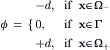
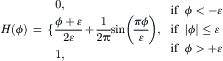
Figure 3.2 shows the domain of interest consisting of two fluids, i.e., the –ve and the +ve fluids, with each occupying the Ω− and the Ω+ regions, respectively. The subregion ΩD with species X concentrated is now contained within the Ω+ region. These fluids are separated by the interface Γ. The evolution of the interface is treated with the level-set method [6]. The level-set function is defined mathematically as
(3.33)
(3.34a)
(3.35)
(3.36a)
(3.36b)
(3.36c)
(3.36d)
The interface is advected by the underlying velocity field  . Its evolution is governed by
(3.37)
Generally,  is nonuniform. Upon advection, ϕ ceases to be a distance function. This is further exacerbated by the unavoidable numerical errors incurred in advecting ϕ.
To maintain ϕ as a distance function after the advection of ϕ via Eqn (3.37), ϕ is set to the steady-state solution of Eqns (3.38)[8]:
(3.38b)
To mitigate the mass loss problem, a particle correction procedure is adopted. Basically, two sets of particles offering subcell resolution are included to keep track of the interface. The particle correction procedure will not be discussed here. Interested readers are referred to [10]. It should be mentioned here again that the level-set method is the authors' personal choice. Other method of treating an evolving interface, e.g., the VOF method [11] and front-tracking method [12] and [13], can also be used.
3.4. Solution Procedure
3.4.1. General transient convection–diffusion equation
The species conservation (Eqn 3.1), the Navier–Stokes (Eqns (3.3) and (3.4)), the energy (Eqn 3.6), electric potential (Eqn 3.23), and magnetic potential (Eqn 3.30) equations can be recast into a general transient convection–diffusion equation of the form
(3.39)
3.4.2. Finite volume formulation
The finite volume method is employed to solve the general transient convection–diffusion equation numerically. This solution procedure follows the idea described in [14] and [15]. Integration of Eqn (3.39) over an arbitrary control volume (CV) gives
(3.40)
Employing Gauss' divergence theorem, the volume integration is converted into a surface integration as
(3.41)
Equation (3.41) states the conservation principle for the quantity Φ within the CV. This equation is applied to every CV to derive discretized governing equations relating the dependent variable of that CV to those of the neighboring CVs. Then, the discretized governing equations express the conservation principle for the CV in a discrete sense.
Application of Eqn (3.41) for a two-dimensional domain will be demonstrated. Equation (3.39) can be expressed in a two-dimensional Cartesian coordinate system as
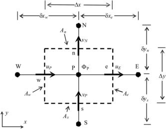
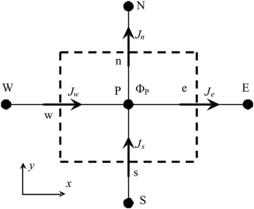
Extension to three dimensions is straightforward. The physical domain is first partitioned into a number of nonoverlapping control volumes (CVs), as shown in Fig. 3.3. A node is located at the center of every CV. For the CV labeled P, the neighboring nodes are denoted as W, E, N, and S as shown in Fig. 3.4. This CV has four boundaries, denoted by e, w, n, and s (with area of Ae, Aw, An, and As, respectively). Δx and Δy are the length and height of the CV. δx and δy are the distances between grid points. The scalar variable, such as pressure, temperature, and electrical potential, are stored at the node P. Velocity components are stored at the CV boundaries. While u is staggered half a CV to the left, v is staggered half a CV downward. A staggered grid is adopted to avoid the check-board distribution of the pressure field. The discrete form of Eqn (3.41) can then be written as:

(3.43)

The source term S in Eqn (3.41) is linearized as
(3.44)
The convective terms are modeled using the first-order upwind scheme as
(3.45a)
(3.45b)
(3.45c)
(3.45d)
(3.46a)
(3.46b)
(3.46c)
(3.46d)
(3.47a)
(3.47b)
(3.47c)
(3.48a)
(3.48b)
(3.48c)
The diffusion coefficients at the interface in Eqn (3.47), i.e., Γe, Γw, Γn, and Γs, are determined using a harmonic mean approach. Upon substitution of Eqns (3.45) and (3.46) into Eqn (3.43), we have
(3.49)

(3.50)
To enforce continuity, the continuity equation has to be considered in the discretization of the general transport equation. For this purpose, the continuity equation (Eqn 3.3) is similarly integrated over the CV to give
(3.51a)
(3.51b)
(3.52)
(3.53b)
(3.53c)
(3.53d)
(3.53e)
(3.53f)
(3.53g)
(3.53h)
3.4.2.1. Higher-order schemes
In the above discussion, the convective terms in Eqn (3.43) are modeled using a first-order upwind scheme (Eqn 3.45). The first-order upwind scheme is numerically too diffusive. Higher-order scheme is then introduced. The convection term is modeled using a second-order upwind scheme with flux limiters. This is achieved easily within the present framework by employing first-order upwind scheme with an additional source term to increase its accuracy to second order via deferred correction approach. An additional source term SDC, included into SC (Eqn 3.53h), is given as [15]
(3.54a)
(3.54b)
(3.54c)
(3.54d)
(3.54f)
(3.54g)
(3.54h)
(3.54i)
(3.55)
(3.56)
3.4.2.2. Remarks
The finite volume integration for the general transient convection–diffusion equation (Eqns (3.39) and (3.40)) is based on the CV centered at the node (Fig 3.5). Similar finite volume integration for the Navier–Stokes equations, although based on staggered CVs, can be made. In the solution of the Navier–Stokes equations, the velocity and pressure have to be coupled. This velocity–pressure coupling is handled with the SIMPLER algorithm [14].
Depending on the design of the micromixer, the domain of interest can be of various geometries. To create the domain of various geometries within the current computational framework, the block-off region approach of [14] can be used.
For two-fluid flows, the harmonic mean (Eqn 3.34b) will be used to determine the relevant diffusion coefficient in Eqn (3.39). These are viscosity in the momentum equations (Eqn 3.4), thermal conductivity in the energy equation (Eqn 3.6), permittivity in Gauss' law for electric field (Eqn 3.23), and relative permeability in Gauss' law for magnetic field (Eqn 3.30).
To capture the evolving interface between two immiscible fluids accurately, the level-set method requires higher-order numerical schemes. The evolution of the level-set function (Eqn 3.37) and its redistancing (Eqn 3.38) are spatially discretized with WENO5 [20] and advected using TVD-RK2 [21]. These schemes are computationally intensive. To reduce the computational effort, the level-set method is implemented in a narrow-band procedure [9] where the level-set function is solved only within a band of certain thickness from the interface. This reduces one order of computational effort.
3.4.3. Solution algorithm
The overall solution procedure is as follows: Given known  ,
,  ,
,  ,
,  ,
,  ,
,  , and
, and  at time t, evolve the solution to
  ,
,  ,
,  ,
,  ,
,  ,
,  and
and  at time t+Δt.
1. Set  .
.
3. Calculate the properties of the fluid using Eqn (3.34).
4. Solve for concentration field cn+1 from Eqn (3.1).
6. Solve for the temperature field Tn+1 from Eqn (3.6).
7. Solve for the electric field  from Eqn (3.23).
8. Solve for the magnetic field  from Eqn (3.30).
9. Repeat steps (2) and (8) until the solution converges.
10. Repeat steps (1) and (8) for all time steps.
3.5. Verifications and Validations
The presented solution procedure has to be validated before it can be used. The first verification is made for the solution of the general transient convection–diffusion equation (Eqn 3.42). The procedure follows that of the “method of manufactured solution”[22]. Since the species conservation (Eqn 3.1), the energy (Eqn 3.6), electric potential (Eqn 3.23), and magnetic potential (Eqn 3.30) equations have a similar form, the same method also verifies the solution procedure for these equations. Then, the solution of the Navier–Stokes equations (Eqns (3.3) and (3.4)) is validated against the case of lid-driven cavity flow. The implementation of the level-set method (Eqns 3.37 and 3.38) is validated against the case of a bubble rising in a container partially filled with a heavier medium.
3.5.1. Verification – solution procedure of the general transient convection diffusion equation
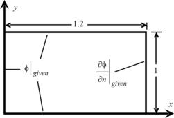
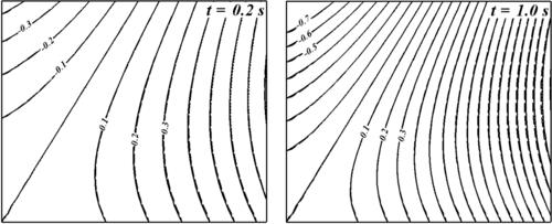
Figure 3.6 shows a rectangular domain in which the solution of the general transient convection–diffusion equation (Eqn 3.42) is sought. In the actual solution of Eqn (3.42), the velocity is known from the Navier–Stokes equations. Therefore, for verification purpose, the velocity is assumed to be known. The velocity components are u=y and v=x. The density and diffusion coefficients are set to ρ=1 and Γ=xy, respectively. There is a source term within the rectangular domain of
(3.57)
(3.58)
For initial condition, ϕ=0 in the whole domain. For the boundary conditions, the value of ϕ is given, except at the right boundary, i.e., x=1.2, where Neumann boundary condition is enforced. Solutions were made using two different meshes, i.e., 24×20 CVs with Δt=0.010 s and 48×40 CVs with Δt=0.005 s. These solutions are shown in Fig. 3.7. A mesh of 24×20 CVs with Δt=0.010 s is sufficient to achieve mesh-independent solution. The predicted solutions agree very well with the exact solution of Eqn (3.58).
3.5.2. Validation – solution procedure of the Navier–Stokes equations
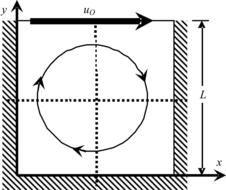
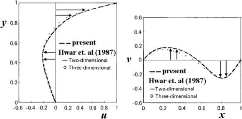
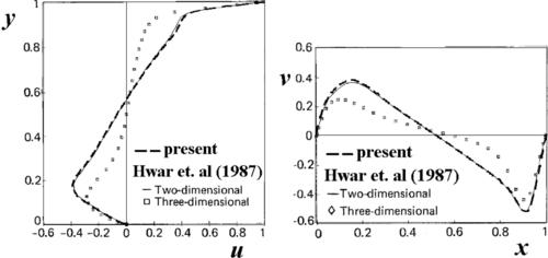
Figure 3.8 shows a fluid within a square cavity. There is a lid at the top of the cavity. The lid is driven at a constant velocity of uo. The motion of the lid transfers momentum to the fluid through the effect of viscosity. This leads to a circulatory motion of the fluid in the cavity. The flow is governed by one dimensionless number, i.e., the Reynolds number  . The u-velocity and v-velocity profiles along the dotted lines of y=L/2 and x=L/2, respectively, are compared to the two-dimensional solution of [23]. FIGURE 3.9 and FIGURE 3.10 show the comparisons for Re=100 and Re=1000, respectively. The predicted velocity profiles agree well with those of [23] for both Reynolds numbers. With these comparisons, the present solution procedure of the Navier–Stokes equations is validated.
3.5.3. Validation – solution procedure of the level-set method
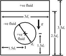
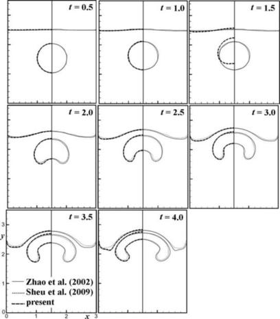
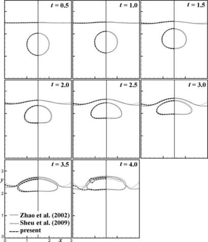
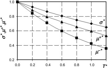
The problem of a rising bubble in a container partially filled with a heavier fluid, as depicted in Fig. 3.11, is considered in this validation exercise. The diameter of the bubble is dc=1.0. As the bubble rises, the bubble itself deforms, thereby deforming the free surface in the process. Therefore, both the bubble interface and the free interface are of interest. The governing dimensionless numbers are the density ratio (ρ∗=ρ−/ρ+), the viscosity ratio (μ∗=μ−/μ+), the Reynolds number  , and the Eotov number
  . These dimensionless parameters are set to ρ∗=2, μ∗=2, and Re=200 in this validation exercise. Two cases of different Eo are considered, i.e., Eo=∞ and 10. The case of Eo=∞ corresponds to the situation without surface tension. FIGURE 3.12 and FIGURE 3.13 show the solution obtained with the present approach compared against to those of [24] and [25]. The agreement between these solutions is reasonably well and validates the present solution procedure of the level-set method. It is pointed out that the solutions of [24] and [25] for Eo=∞ at t=1.0 and t=1.5 are identical. The authors believe that the solutions given in [24] and [25] at t=1.5 are in fact those at t=1.0. The present solution for t=1.5 is shown.
3.6. Examples
3.6.1. Mixing in a micro-enclosure
Figure 3.14 shows a two-dimensional square enclosure. Initially, the species X is concentrated in the dotted region. The rest of the enclosure does not contain species X. Species X spreads to the rest of the domain by molecular diffusion. The prediction of the mixing process of species X is described in this section. The transport of species X is only governed by the species conservation equation (Eqn 3.1).
The diffusion coefficient is set to D=10−9 m2/s. As the wall of the enclosure is impermeable to the transport of species X, the zero-flux condition  is applied to all the four walls. Figure 3.15 shows the concentration of species X at different time t. The increment between two iso-contours for the concentration is 0.1. A mesh of 20×20 CVs with Δt=10−3 gives mesh-independent solution. Species X spreads toward the walls of the enclosure, i.e., in the direction of lower concentration. The effect of the wall is only obvious after t=0.16 s.

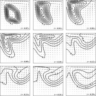
3.6.2. Mixing in a lid-driven microcavity
Figure 3.16 shows a lid-driven microcavity. The dotted square region within the cavity contains a concentrated species X. There is no species X in the rest of the cavity. The motion of the lid (uo=0.003 m/s) generates a circulatory motion within the cavity. Therefore, besides molecular diffusion, species X is convected by the flowing fluid. The convective transport of species X can greatly enhance mixing. This problem is governed by the species conservation (Eqn 3.1) and the Navier–Stokes (Eqns (3.3) and (3.4)) equations. The diffusion coefficient is set to D=10−9 m2/s. As the lid and the three walls of the cavity are impermeable to the transport of species X, the zero-flux condition is applied at these boundaries. For the Navier–Stokes equations, the properties of water are used, i.e., μ=10−3 Pa s and ρ=1000 kg/m3. No-slip condition is enforced at the lid and the three walls. The velocity u=uo is given at the lid as the boundary condition. The concentration of species X and the fluid velocity are shown in Fig. 3.17. The effect of the velocity field on the concentration distribution of species X is dominant.
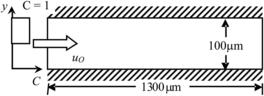
3.6.3. Mixing in a straight microchannel
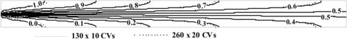
Figure 3.18 shows a straight microchannel. Water flows into the microchannel at the inlet carrying a nonuniform concentration of species X. Mixing of species X then occurs in the microchannel. This problem is governed by the species conservation (Eqn 3.1) and the Navier–Stokes (Eqns (3.3) and (3.4)) equations. The diffusion coefficient is set to D=10−9 m2/s. For species X, at the inlet, the concentration of species X is nonzero only at the upper half of the microchannel. The zero-flux condition is applied at both the upper and lower walls. At the outlet, zero-gradient condition is enforced. For the Navier–Stokes equations, the properties of water are used. A velocity of uo=0.01 m/s is set at the inlet. No-slip condition is enforced at the walls. Outflow boundary condition is used at the outlet. A steady-state solution is sought. Figure 3.19 shows the steady-state concentration distribution in the microchannel. The results show that species X diffuses into the fluid in the lower half of the microchannel.
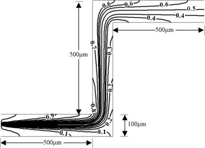
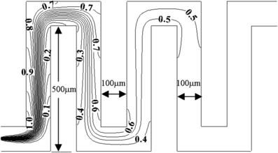
3.6.4. Mixing in winding microchannels
The same mixing problem of Section 3.6.3 is considered for two different winding microchannels. These are a double-bend microchannel and a serpentine microchannel, depicted respectively in FIGURE 3.20 and FIGURE 3.21. The steady-state concentration distributions are shown in these figures. In terms of compactness, the serpentine microchannel offers more turnings to enhance mixing of species X. In this configuration, species X is considered homogenously mixed after the third ‘U’ turns.
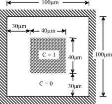
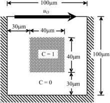
3.6.5. Mixing within a droplet flowing in a straight microchannel
Figure 3.22 shows a water droplet carried by oil flowing in a straight microchannel. The droplet of radius R1=25 µm is initially located at (50, 50). The lower half of the droplet contains a nonzero concentration of species X (c=1.0). There is no species X in the rest of the droplet. Since water and oil are immiscible, species X can only be convected or diffuse within the droplet. This problem is governed by the species conservation (Eqn 3.1) and the Navier–Stokes (Eqns (3.3) and (3.4)) equations. The level-set method is required to capture the interface of the droplet.
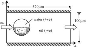
For this demonstration, the diffusion coefficient is set to D=10−8 m2/s. The concentration of species X is set to 0 at the inlet. At the outlet, it is set to zero gradient with the assumption of pure convective transport of species X. Zero-flux condition is enforced at both the upper and the lower walls of the microchannel.
For the Navier–Stokes equation, the properties of oil and water are used  . For flow in microscale, the effect of density is normally not important, and the density of oil is slightly lower than that of water. Thus, identical density is used for both liquids. The surface tension between water and oil is set to σ=3.65×10⁻³ N/m. The inlet velocity is specified as uo=0.003 m/s. Outflow boundary condition is used at the outlet. At the walls, no-slip condition is enforced.
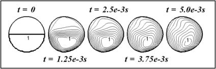
In the solution of the species conservation equation, a second-order upwind method with Superbee flux limiter is employed for the convective terms. Even with a second-order scheme, species X diffuses out of the droplet during the solution process because of the inherited numerical diffusion of the scheme. This phenomenon is purely a numerical artifact and therefore is not physical. An even higher-order scheme can be an alternative to alleviate this problem. However, the authors choose to adopt a simpler approach, though less mathematically sophisticated. The amount of species X diffused out of the droplet is redistributed back into the droplet uniformly by making an appropriate correction to c within the droplet and setting c=0 in the oil region at every time step.
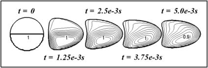
Figure 3.23 shows the concentration of species X in the droplet as it is carried by the flow. The droplet deforms, although slightly, in the flow due to stresses exerted on it by the flowing oil. Figure 3.24 shows the case of a much lower surface tension of σ=3.65×10⁻⁴ N/m. A lower surface tension can be achieved physically, for example, by adding suitable surfactant. With a lower surface tension, the deformation of the droplet is much larger. The deformation of the droplet by the flow generates a larger v-velocity component. This helps mixing of species X within the droplet. The highest concentration at t=5.0×10⁻³ s is reduced from c=1 to c=0.9.
3.6.6. Mixing within a droplet flowing through a micro-U-bend
Figure 3.25 shows a water droplet carried by oil flowing in U-bend. The droplet of radius R1=35μm is initially located at (50, 50). The lower half of the droplet contains a nonzero concentration of species X(c=1.0). There is no species X in the rest of the droplet. This problem is governed by the same equations in Section 3.6.5. The diffusion coefficient is again set to D=10−8 m2/s. The inlet velocity is specified as uo=0.003 m/s. The evolutions of the droplet for σ=3.65×10⁻³ and σ=3.65×10⁻⁴ N/m are shown in FIGURE 3.26 and FIGURE 3.27, respectively. For the case of σ=3.65×10⁻⁴ N/m, the deformation of the droplet is large, especially when the droplet negotiates the bend. The droplet breaks with a smaller satellite droplet formed trailing the main droplet.
 |
| FIGURE 3.26 |
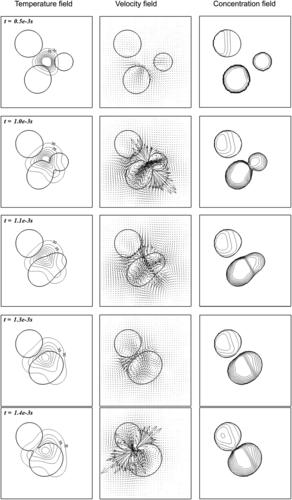
3.6.7. Mixing in three thermocapillary merged droplets
Figure 3.28 shows a square enclosure containing three water droplets suspended in oil. These droplets of radii R1=15, R2=15, and R3=10 µm are located initially at (40, 30), (30, 70), and (70, 50), respectively. The concentrations of species X in droplets 1 and 3 are c1=1.0 and c3=0.5, respectively. For droplet 2, only the left half of the droplet contains species X of concentration c2=0.3. There is no species X in the right half of droplet 2.
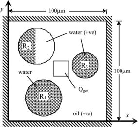
Initially, the temperature of both water droplets and oil is at To=25 °C. Heat is being generated in a localized manner within the square-shaped region at the center of the enclosure. This can be achieved conveniently, for example, by laser heating. The volumetric heat generation is Qgen=1 W/m3. With heat generation, the temperature in the enclosure then varies both temporally and spatially. This affects the properties of oil and water. The temperature-dependent properties of oil and water normalized with their corresponding values at To=25 °C are re-fitted as polynomial functions from the data in [26] as:
(3.59a)
(3.59b)
(3.59d)
(3.59e)
(3.59f)
(3.59g)
The variations of these properties as temperature changes are plotted in Fig. 3.29. Of particular interest is the variation of surface tension. This spatial variation of surface tension induced by the temperature field generates an additional Marangoni force (second term in Eqn 3.36a, i.e.,  ) that drives flows. The net effect of the Marangoni force, in this context, is to drive the microdroplets dynamically toward the region of higher temperature. This temperature-induced phenomenon is called thermocapillary effect.
For the situation considered, the variations of density, specific heat, and thermal conductivity with temperature are not considered. The densities of both fluids are set to be identical 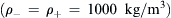 . The specific heats of oil and water are cp−=1700J/(kg°C) and cp+=4200J/(kg°C), respectively. For thermal conductivity, k−=0.17W/(m°C) and k+=0.6W/(m°C).
This problem is governed by the species conservation (Eqn 3.1), the Navier–Stokes (Eqns (3.3) and (3.4)), and the energy (Eqn 3.6) equations. Again, the level-set method is required to capture the interface of the droplet. For the species conservation equation, the diffusion coefficient is set to D=10−8 m2/s. The zero-flux condition is applied at the four walls of the enclosure. For the Navier–Stokes equations, a no-slip condition is enforced at the four walls of the enclosure. For the energy equation, the four walls are maintained at T=25°C.
The merging process of the droplets is depicted in Fig. 3.30. The temperature, velocity, and concentration fields are plotted sequentially in the first, second, and third columns, respectively. It can be observed that the three droplets are driven toward the center of the enclosure where the temperature is highest. Because of the proximity of droplets 1 and 3 and the smaller size of droplet 3, these two droplets are first merged (t=1.0×10⁻³ s). Then surface tension acts to minimize the surface area of the merged droplet by restoring the droplet into a more circular shape (t=1.3×10⁻³). This newly merged droplet is then merged with droplet 2, forming an even larger droplet (t=1.4×10⁻³). At the end of the merging process, the concentration of species X in this newly formed droplet has yet not achieved equilibrium. Mixing of species X continues within this newly formed droplet.
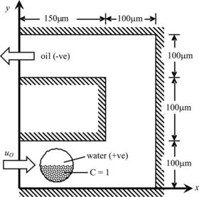
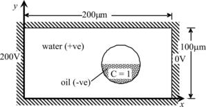
3.6.8. Mixing within a droplet driven by electroosmotic flow in an enclosure
Figure 3.31 shows an enclosure containing an oil droplet suspended in water. Initially, the droplet of radius R=22.5μm is located at (150, 45). Only the lower half of the droplet contains species X. A voltage difference of 200V is applied across the two ends of the enclosure. An electroosmotic flow of water is induced and hereby set the droplet into motion.
This problem is governed by the species conservation (Eqn 3.1), the Navier–Stokes (Eqns (3.3) and (3.4)), and electric potential (Eqn 3.23) equations. The level-set method is required to capture the interface of the droplet.
For the species conservation equation, the diffusion coefficient is set to D=10−8 m2/s. Zero-flux condition is applied at the four walls. For the Navier–Stokes equation, the properties of oil and water are used  . The surface tension between water and oil is set to σ=3.65×10⁻³ N/m. The Helmholtz–Smoluchowski slip velocity (Eqn 3.25) is imposed at the upper and the lower walls. No-slip condition is enforced at both ends of the enclosure.
For the electric field, the permittivities of water and oil are set to ɛe+=80.1ɛo and ɛe−=3.1ɛo, respectively, where the permittivity of vacuum is given by ɛo=8.854×10⁻¹² F/m. The zeta potential of the wall is ζ=−102×10−3 V. Both the upper and the lower walls are insulated. The electric potentials at the right and left ends of the enclosure are maintained at 200V and 0V, respectively.
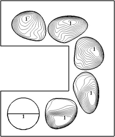
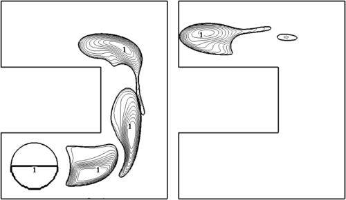
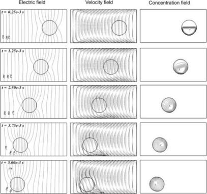
Figure 3.32 shows the electric, velocity, and concentration fields generated by electroosmotic effect. It induces a circulatory flow within the enclosure. The droplet is driven toward the left end of the enclosure. When approaching the left end of the enclosure, the droplet moves toward lower wall as the flow of the carrier fluid, i.e., water, changes direction. This induces a circulatory flow within the droplet (t=3.75×10⁻³ and t=5.0×10⁻³), proving additional stirring to enhance mixing of species X. The deformation of the droplet is minimal, given the strong effect of surface tension.
3.6.9. Mixing within a ferrofluid droplet
Figure 3.33 shows a ferrofluid droplet neutrally buoyant in oil in an enclosure. The ferrofluid droplet has a radius of R=70 µm. It is located initially at the center of the enclosure. Only the upper half of the droplet contains a nonzero concentration of species X (c=1.0). A magnetic field intensity of  is impulsively applied across the ferrofluid droplet at t=0 s.
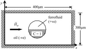
This problem is governed by the species conservation (Eqn 3.1), the Navier–Stokes (Eqns (3.3) and (3.4)), and magnetic potential (Eqn 3.30) equations. To capture the interface of the droplet, the level-set method is employed.
For the species conservation equation, the diffusion coefficient is set to D=10−8 m2/s. A zero-flux condition is set at the walls. The ferrofluid is water based. The properties of water were used as approximations. The surface tension between ferrofluid and oil is set to σ=3.65×10⁻⁴ N/m. A lower surface tension is used so that larger deformation of the droplet can be achieved.
For the magnetic potential equation, the relative permeability, i.e., 1+χ, is evaluated using Eqn (3.34b) as:
(3.60)
(3.61a)
(3.61b)
Accordingly, the momentum equation has to be modified to include the magnetic force in the form of Eqn (3.32). For the present two-fluid system, the magnetic force  can be further reduced to [4] and [5]
(3.62a)
(3.62b)
(3.62c)
Equation (3.62c) is derived from Eqn (3.60). In the solution of the fluid transport equations, no-slip boundary condition is applied at the four walls.
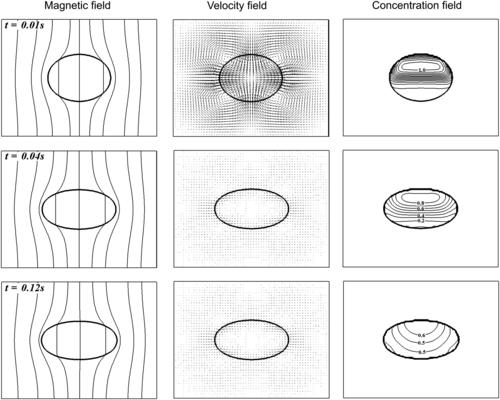
Figure 3.34 shows the magnetic, velocity, and concentration fields generated by the applied magnetic field. The applied magnetic force stretches the droplet in the direction of the applied field. Driven by the applied magnetic field, the droplet evolves dynamically to its equilibrium shape where the magnetic force is balanced by the surface tension force and the velocity field dies down in the process. Obviously, the droplet has not achieved this equilibrium shape at t=0.12 s. The twofold symmetries of the flow field, in this case, help to redistribute species X within the droplet and enhance mixing.
3.7. Concluding Remarks
This chapter presents a general computational framework to investigate microscale transport processes, in particular mixing. With the solution procedure in the framework verified and validated, the present framework is employed for simulating various two-dimensional mixing problems, including those with temperature, and electric and magnetic fields. Although demonstrated only for two-dimensional problems, the present framework can be readily extended to three-dimensional problems without any complication.
References
[1] Bird, R.B.; Stewart, W.E.; Lightfoot, E.N., Transport Phenomena. Second ed (2007) John Wiley & Sons Inc, New York.
[2] Paris, D.T.; Hurd, F.K., Basic Electromagnetic Theory. (1969) McGraw-Hill Inc, New York.
[3] Edward, J.R.; Michael, J.C., Electromagnetics. (2001) CRC Press LLC, Boca Raton, Florida.
[4] Rosensweig, R.E., Ferrohydrodynamics. (1985) Cambridge University Press, Cambridge.
[5] Bhattacharjee, P.; Riahi, D.N., Numerical Study of Surface Tension Driven Convection in Thermal Magnetic Fluids. IDEALS TAM Reports 1081 (2005) University of Illinois;http://hdl.handle.net/2142/339.
[6] Osher, S.; Sethian, J.A., Fronts propagating with curvature-dependent speed: Algorithms based on Hamilton-Jacobi formulations, J. Comput. Phys. 79 (1988) 12–49.
[7] Brackbill, J.U.; Kothe, D.B.; Zemach, C., A continuum method for modelling surface tension, J. Comput. Phys. 100 (1992) 335–354.
[8] Sussman, M.; Smereka, P.; Osher, S., A level set approach for computing solution to incompressible two-phase flow, J. Comput. Phys. 114 (1994) 146–159.
[9] Peng, D.; Merriman, B.; Osher, S.; Zhao, H.; Kang, M., A PDE-based fast local level-set method, J. Comput. Phys. 155 (1999) 410–438.
[10] Enright, D.; Fedkiw, R.; Ferziger, J.; Mitchell, I., A hybrid particle level set method for improved interface capturing, J. Comput. Phys. 183 (2002) 83–116.
[11] Hirt, C.W.; Nichols, B.D., Volume of fluid (VOF) method for the dynamics of free boundaries, J. Comput. Phys. 39 (1981) 201–225.
[12] Glimm, J.; Grove, J.W.; Li, X.L.; Shyue, K.M.; Zeng, Y.; Zhang, Q., Three-dimensional front-tracking, SIAM J. Sci. Comput. 19 (1998) 702–723.
[13] Unverdi, S.O.; Tryggvason, G., A front-tracking method for viscous, incompressible, multi-fluid flows, J. Comput. Phys. 100 (1992) 25–37.
[14] Patankar, S.V., Numerical Heat Transfer and Fluid Flow. (1980) Hemisphere Publisher, New York.
[15] Versteeg, H.K.; Malalasekera, W., An Introduction to Computational Fluid Dynamics: the Finite Volume Method. Second ed (2007) Prentice Education Limited, England.
[16] van Leer, B., Towards the ultimate conservative difference scheme. V. A second-order sequel to Godunov's method, J. Comput. Phys. 32 (1979) 101–136.
[17] Sweby, P.K., High resolution schemes using flux limiters for hyperbolic conservation laws, SIAM J. Num. Anal. 21-5 (1984) 995–1011.
[18] P.L. Roe, M.J. Baines, Algorithms for advection and shock problems, in: Proc. of the 4th GAMM Conf. on Num. Meth. in Fluid Mech., Paris, France, Oct. 7–9, 1981.
[19] P.L. Roe, Some contributions to the modelling of discontinuous flows, in: Proc. of the 15th Summer Seminar on App. Math., La Jolla, CA, Jun. 27–Jul. 8, 1983.
[20] Jiang, G.S.; Peng, D., Weighted ENO schemes for Hamilton–Jacobi equations, SIAM J. Sci. Comput. 21 (2000) 2126–2143.
[21] Shu, C.W.; Osher, S., Efficient Implementation of Essentially Non-Oscillatory Shock Capturing Schemes, J. Comput. Phys. 77 (1988) 439–471.
[22] Roache, P.J., Code verification by the method of manufactured solution, J. Fluids Eng. 124 (2002) 4–10.
[23] Hwar, C.K.; Hirsh, R.S.; Taylor, T.D., A pseudospectral method for solution of the three-dimensional incompressible Navier–Stokes equations, J. Comput. Phys. 70 (1987) 439–462.
[24] Sheu, T.W.H.; Yu, C.H.; Chiu, P.H., Development of a dispersively accurate conservative level set scheme for capturing interface in two-phase flows, J. Comput. Phys. 228 (2009) 661–686.
[25] Zhao, Y.; Tan, H.H.; Zhang, B., A high-resolution characteristics-based implicit dual time-stepping VOF method for free surface flow simulation on unstructured grids, J. Comput. Phys. 183 (2002) 233–273.
[26] Nguyen, N.T.; Ting, T.H.; Yap, Y.F.; Wong, T.N.; Chai, J.C., Thermally mediated droplet formation in microchannels, Appl. Phys. Lett. 91 (2007) 084102.
..................Content has been hidden....................
You can't read the all page of ebook, please click here login for view all page.