
Chapter 5. Micromixers based on molecular diffusion
Chapter Outline
5.1. Parallel Lamination163
5.2. Sequential Lamination171
5.3. Sequential Segmentation173
5.4. Segmentation Based on Injection175
5.5. Focusing of Mixing Streams177
5.6. Gradient Generator Based on Diffusive Mixing187
References193
The final stage in all micromixer types is molecular diffusion. This chapter discusses micromixers that rely entirely on diffusive transport. As pointed out in Chapter 2, diffusive mixing can be improved by increasing the interfacial area between the solute and solvent or by decreasing the striation thickness of these two phases. Based on Fick's law, a large interfacial area, a large gradient, and a large diffusion coefficient can lead to a high diffusive flux. The small mixing length in microscale actually leads to a higher concentration gradient and is thus advantageous for diffusive mixing. Because diffusion coefficient is a material constant, larger diffusion coefficients can only be achieved by a higher temperature and a lower viscosity. However, the resulting improvement in diffusive flux based on temperature and viscosity is not significant. Thus, mixing in micromixers based on molecular diffusion can only be optimized by geometrical designs for decreasing the striation thickness. In this chapter, the basic concepts for decreasing the striation thickness include parallel lamination, sequential lamination, sequential segmentation, segmentation based on injection, and focusing.
The final stage in all micromixer types is molecular diffusion. This chapter discusses micromixers that rely entirely on diffusive transport. As pointed out in Chapter 2, diffusive mixing can be improved by increasing the interfacial area between the solute and solvent or by decreasing the striation thickness of these two phases. Based on Fick’s law, a large interfacial area, a large gradient, and a large diffusion coefficient can lead to a high diffusive flux. The small mixing length in microscale actually leads to a higher concentration gradient and is thus advantageous for diffusive mixing. Because diffusion coefficient is a material constant, larger diffusion coefficients can only be achieved by a higher temperature and a lower viscosity. However, the resulting improvement in diffusive flux based on temperature and viscosity is not significant. Thus, mixing in micromixers based on molecular diffusion can only be optimized by geometrical designs for decreasing the striation thickness. In this chapter, the basic concepts for decreasing the striation thickness include parallel lamination, sequential lamination, sequential segmentation, segmentation based on injection, and focusing.
5.1. Parallel Lamination
5.1.1. Mixers based on pure molecular diffusion
Parallel lamination increases the interfacial area and decreases the striation thickness by splitting the solute and the solvent each into n substreams and rejoining them later in a single stream. Compared to a parallel mixer with two substreams, the mixing time or the required channel length can be reduced by a factor of n2.
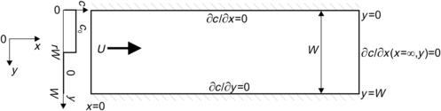
The simplest parallel lamination mixer is a straight channel with two inlets. The two inlets form a Y-shape or a T-shape. Thus, this mixer is often called Y-mixers or T-mixers. The following analytical model describes the concentration distribution inside the straight channel. The model is two dimensional and assumes that the microchannel is flat (Fig. 5.1). The height H of a flat channel is much smaller than its width W (H≪W). This model was solved numerically in Section 3.6.3.
 |
| FIGURE 5.1 |
Earlier, Example 2.4 showed that different viscosities will cause different flow velocities on each side of the mixing channel. The mismatch in velocity will certainly affect the convective transport in the mixing channel. In the following model, the mixing streams are assumed to have the same viscosity and the same mean velocity  to keep the model simple and analytically solvable. The mixer is a long channel with a width W. The inlets are defined with the inlet boundary on the left, while the outlet is defined with the exit boundary on the right side of the model. The inlets consist of a solute stream and a solvent stream. The solute stream has a concentration of c=c0 and a mass flow rate of
  . The solvent stream has a concentration of c=0 and a mass flow rate of
  . At an infinite exit position, the two streams are well mixed such that no concentration gradient exists (∂c/∂x=0, ∂c/∂y=0).
With the above assumptions, the transport Eqn (2.22) can be reduced to the steady-state two-dimensional form:
(5.1)
Introducing the dimensionless spatial variables x∗=x/W, y∗=y/W, the dimensionless concentration c∗=c/c0, and the Peclet number  , the transport equation has the dimensionless form:
(5.2)
The corresponding boundary conditions for the inlets are
The exit boundary condition at (x∗=∞) is
(5.4)
The wall conditions are
(5.5)
The wall condition (5.5) is also the symmetry condition in the case of mixing with multiple streams. Thus, this model can also be used for describing parallel lamination with more than two inlets. Using separation of variables and the corresponding boundary conditions (5.3), (5.4) and (5.5), the dimensionless concentration distribution in the mixing channel is
(5.6)
The function of the concentration distribution (5.6) is described by a cosine function of the y∗-axis and an exponential function of the x∗-axis. It is clear that complete mixing is determined by the Peclet number in the exponential term. A large Peclet number requires a long mixing length along the x∗-axis to make the exponential term approach zero. Physically, a large Peclet number means that convection is dominant over molecular diffusion and it would take longer for the solute to diffuse in the transversal direction across the mixing channel.
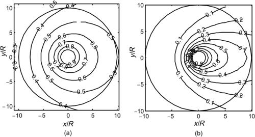
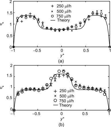
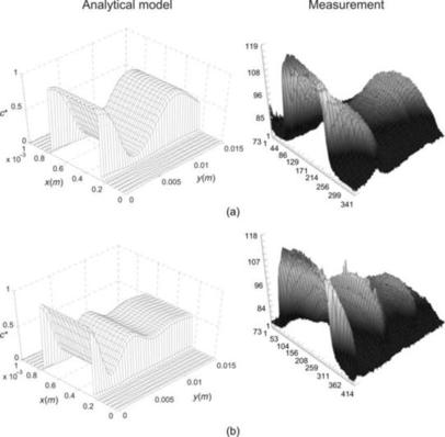
The solution of concentration distribution (5.6) clearly shows that mixing can be improved by operating the mixer at a small Peclet number. Since diffusion coefficient is a material property, a small Peclet number can be achieved with a low flow velocity or a small width. Small width and a thin striation thickness shorten the transversal transport of the solute. The simplest way to achieve thin striations is to split the solvent and the solute into multiple mixing streams. As mentioned above, solution (5.6) can also be extended to the case of multiple mixing streams. The wall boundary condition is identical to the symmetry condition in the middle of each stream. Thus, the concentration distribution (5.6) can be extended periodically along the transversal y- or y∗-direction. Considering the distance between two neighboring concentration extrema Wmin,max, the Peclet number is evaluated as Pe=UWmin,max/D. Figure 5.2 shows the typical theoretical and experimental results in a parallel lamination micromixer with two or three streams, respectively. The case of mixing with three streams is often referred to as hydrodynamic focusing, where the width of the middle stream and consequently the mixing time can be controlled by the sheath streams.
 |
| FIGURE 5.2 |
For mixing channels with aspect ratio on the order of unity, the velocity profile across the channel width is parabolic and not uniform as assumed for the analytical model. The transport equation has the form
(5.7)
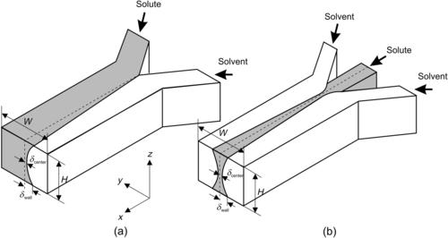
The dispersion effect in parallel lamination is illustrated in Fig. 5.3. Due to the no-slip boundary condition, flow velocity at the channel wall grows from zero to the maximum value at the channel center. Near the channel wall, molecular diffusion dominates over convective transport, leading to faster diffusion of the solvent into the solute and a cross-sectional concentration as depicted in Fig. 5.3 (a). The dispersion effect can be observed directly with confocal microscopy using Fluo-3 and calcium chloride (CaCl2) solution [2]. Fluo-3 is nonfluorescent, but forms with calcium ions into a strongly fluorescent compound. Ismagilov et al. experimentally observed and, using dimensional analysis to Eqn (5.7), derived the following relation between the broadening width δ and other parameters such as axial position x, channel height H, and the mean velocity at the channel center and at the channel wall, respectively:
 |
| FIGURE 5.3 |
In Eqn (5.8), the term  represents the mixing time. For a small channel height (H≪W), the difference between the broadening widths at the wall and at the channel center is quickly equalized due to diffusion in z-direction. The broadening effect is also less dramatic if the mixing time is short. Short mixing time means a high mean velocity , which makes convection dominate over molecular diffusion.
Based on numerical results of Eqn (5.7), the same relation was obtained by Kamholz et al. [3]. The square-root relation at the center of the channel reflects the relation between the required length of the mixing channel and its width Lmixer/W∝PeW (2.200) derived in Section 2.8. The one-third-power relation at the channel wall shows that mixing based on molecular diffusion is better, in reality, due to the distributed velocity profile. According to numerical results presented by Kamholz and Yager [3], relations (5.8) are true for a short distance x close to the channel entrance. At an intermediate distance, the broadening width is proportional to two-thirds power of the distance x. At a long distance, the broadening width at both the wall and the channel center is again proportional to the square root of the distance x.
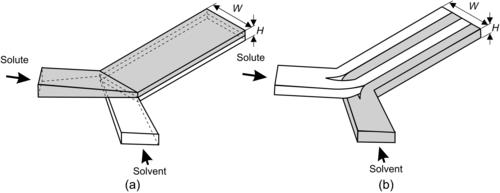
As mentioned earlier, fast mixing is achieved in parallel lamination micromixers by decreasing the mixing path and increasing the contact surface between the solvent and the solute. The simplest parallel lamination micromixers are T-mixers or Y-mixers. If the aspect ratio of the mixing channel is small (W≫H), the inlet streams of a T-mixer can be twisted and laminated as two thin liquid sheets to reduce the mixing path from the channel width W to the channel height H as shown in Fig. 5.4 (a). The interface between the two streams also increases by a factor of W/H. Hinsmannn et al. introduced the streams into the mixing channel through a laminator consisting of many small channels [4]. The laminator keeps the flow at the entrance on their track and minimizes instability.
 |
| FIGURE 5.4 |
The more common technique for shortening the striation thickness is splitting the solute and the solvent into multiple streams and rejoining them through parallel lamination (Fig. 5.4). Combining parallel lamination with geometric focusing can be a powerful concept to improve the micromixer’s performance [5]. Figure 5.5 (a) illustrates this concept. With a large number of streams, the outer streams may experience a sharp bend during the focusing process. At small flow velocities or low Reynolds numbers, the bend has almost no effect on the shape of the lamellae. However, at high Reynolds number on the order of 10 or 100, secondary flow caused by inertial forces (see Section 2.4.2) distorts the shape of the lamellae [6]. Figure 5.5 (b) shows schematically this change of concentration distribution at the cross-section A-A in Fig. 5.5 (a). Inertial effects, which cause recirculation and chaotic advection and improve mixing, are discussed later in Section 5.1.2.
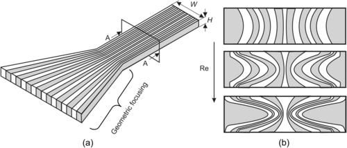 |
| FIGURE 5.5 Parallel lamination with geometric focusing: (a) concept and (b) distortion of the shape of lamellae. (after [6]) |
Splitting the solvent and the solute into multiple streams and rejoining them were realized in an interdigitating manner [7]. Figure 5.6 depicts this mixing concept. Interdigitated lamination offers both thin striation thickness and large interface between the solute and the solvent. The interfacial area can be further increased with the corrugated design as shown in Fig. 5.6 (b). For instance, the design of Bessoth et al. can achieve full mixing with 32 streams only after a few milliseconds [8] and [9].
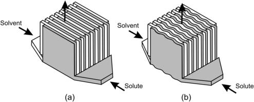 |
| FIGURE 5.6 |
Another concept for reducing the mixing path in parallel lamination micromixers is hydrodynamic focusing. Knight et al. [10] reported a simple mixer with three inlets. The width of the solvent stream in the middle was focused by adjusting the pressure ratio between the sample flow and the sheath flow. Due to the very small focused width of the solvent stream, mixing time can be reduced to a few microseconds [12]. The same configuration of hydrodynamic focusing and mixing was used for cell infection [13]. Flow focusing will be discussed later in a separate section.
5.1.2. Mixers based on inertial and viscoelastic instabilities
According to the dimensionless analysis (2.200) in Section 2.8, the required channel length is proportional to the Peclet number. In most cases, the required channel length is not practical for implementation in miniaturized platforms. A short mixing channel can achieve full mixing at extremely high Reynolds numbers (more than 100) [14] and [15]. Secondary flow and chaotic advection improve mixing by further reducing the mixing path. Because of the required high Reynolds number and the high pressure, this mixing concept can only be implemented in mechanically rigid materials such as silicon, glass [15] and stainless steel. For instance, the mixer reported in [15] needs a flow velocity as high as 7.6 m/s at a pressure of up to 7 bars to achieve Reynolds numbers up to 500. The large velocity gradient in microscale at high Reynolds number leads to the formation of extremely fast vortices. Improved mixing can be achieved with such vortices. Lim et al. [16] created vortices in a diamond-shaped cavity next to a straight microchannel with a flow velocity of 45 m/s. The corresponding Reynolds number, in this case Re=245, is very large for a typical microscale application. Such vortex-based mixers require velocities as high as 10 m/s and pressure up to 15 bars.
Vortices caused by inertial effects can be generated at moderate Reynolds numbers with turns and geometrical obstacles. For instance, a simple 90° bend in the mixing channel can generate vortices at Reynolds numbers above 10 [14]. Mixing is achieved with a single bend at Reynolds numbers higher than 30. Obstacles such as structures on channel wall [17] or throttling the channel entrance [18] can also induce inertial instabilities into the standard T-mixer design. More details about this mixer type are discussed later in Chapter 5.
For simplification in modeling and characterization, most micromixers in this book are assumed to work with Newtonian fluids. As discussed previously, instability in Newtonian flows at high Reynolds number is caused by the competing viscous force and inertial force. Because most micromixers used for biochemical analysis work with relatively low flow rates, the Reynolds number would not be high enough for instability. Flow instabilities at low Reynolds number can be achieved using another force to replace the inertial force. In active micromixers, these forces are induced by external sources and are discussed later in Chapter 7. Diluting a small amount of highly deformable polymers would introduce elasticity to a fluid. This class of fluid is called viscoelastic fluid and belongs to the non-Newtonian fluid family. The elastic forces caused by stretching and recoiling of the polymer molecules can work against the viscous forces to induce instabilities.
The shear stress in viscoelastic fluid does not jump to zero after the disappearance of a driving force. Due to its elastic property, the stress decays with a characteristic time called the relaxation time. In macroscopic mixing devices, the relaxation time is much smaller than the characteristic residence time of the flow. Thus, elastic effect does not affect to a great extent the overall flow behavior. In microscale, the relaxation time and the characteristic residence time of the flow are of the same order. Thus, elastic forces become dominant.
As discussed in Section 2.5, the elastic effect of viscoelastic fluid flow can be characterized by the Weissenberg number, which is the ratio between the relaxation time and the characteristic residence time (2.125). Flows in microchannels have typically low Reynolds numbers and high Weissenberg numbers. The ratio between these two numbers is called the elasticity number (2.127). Because of the low Reynolds number and the high Weissenberg number, elasticity numbers in microchannel can reach up to 100.
Groisman and Steinberg [19] use a mixer design with repeated circular turns to induce viscoelastic instability (Fig. 5.7). Because of the turn, instability is caused by a complex interplay between inertial, viscous, centrifugal, and viscoelastic forces. With a cross-section of 3 mm×3 mm, the mixing channel is large for common micromixers. The viscoelastic fluid is a solution of 80 p.p.m polyacrylamide (PAA, molecular weight of 1.8×10⁷), 65% saccharose, and 1% NaCl in water. Good mixing was reported at an axial distance of about 41 cm from the entrance. However, with the relatively sharp turns W/R=3/4.5, mixing can be achieved with Dean vortices as well (see Section 6.1.3).
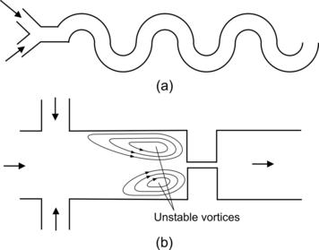 |
| FIGURE 5.7 |
Gan et al. [20] utilized viscoelastic instability at a sudden contraction to improve mixing. Good mixing was achieved at low Reynolds numbers (Re<1). The device was made of silicon. The microchannels have a depth of 150 μm. The sudden constriction has dimensions of 1000 μm: 125 μm: 1000 μm. The micromixer has the flow-focusing configuration. The fluid of the middle stream consists of 1 wt% polyethyleneoxide (PEO) in 55 wt% glycerol water. The fluid of the side streams consists of 0.1 wt% PEO in water. For a total flow rate of 12 ml/h, the corresponding Peclet, Reynolds, Weissenberg, and elasticity numbers are Pe=49.4×10⁶, Re=0.06, We=278, and El=5070, respectively. The very large elasticity number shows that inertial forces are negligible compared to elastic forces. At this high elasticity number, unstable vortices appear before the constriction as depicted in Fig. 5.7 (b). The asymmetric vortices oscillate from side to side leading to chaotic advection. Mixing was improved further by molecular-scale effects caused by stretched and collapsed polymer molecules.
5.2. Sequential Lamination
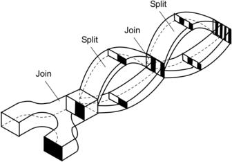
Sequential lamination segregates the joined stream into two channels and rejoins them in the next transformation stage (Fig. 5.8). Because of these characteristics, sequential lamination is also called split-and-recombine (SAR) concept [21]. Because the SAR process is similar to the stretching and folding of mixing fluids, this concept is also called the Baker transformation or the Bernoulli transformation [22] and [23]. Considering the time-dependent striation thickness w(t) with initial value w(0) = W, where W is the width of the microchannel, the decrease of striation thickness is determined by the function α(t):
(5.9)
In chaotic advection, the function α(t) is also called the stretching function and is positive. In the local coordinate system of the striation, the diffusion process is described by the normalized diffusion equation:
(5.11)
(5.12)
The penetration distance δ in the (x∗, t∗) space is given by δx∗∼t∗1/2. Thus, the relation for the penetration distance δx in the (x, t) space is
(5.13)
Mixing is complete if δx=Wfinal when the diffusive penetration distance is on the same order of the striation thickness:
(5.14)
The value of α is inversely proportional to the shear rate  ; thus, PeW∝αW2/D. At the fully mixed state [exp(2αtfinal)≫1], the required channel length of the mixer would be
(5.15)
The transformations described above can be achieved either by sequential lamination or by chaotic advection. Sequential lamination can be implemented by forced splitting and lamination or by chaotic advection. Forced splitting and lamination are achieved at low Reynolds number with a complex channel design. Chaotic advection occurs at a higher Reynolds number and will be discussed later in Chapter 6. The implementation of the concept depicted in Fig. 5.8 is referred to as sequential lamination with vertical lamination and horizontal splitting. Similar transformations can be achieved with horizontal lamination and vertical splitting. This mixing concept requires relatively complicated three-dimensional fluidic structures. According to (2.201) and (2.202), the sequential concept results in much faster mixing compared to the parallel concept with the same device area. Due to their complex geometry, most of the reported sequential lamination mixers were fabricated in silicon, using bulk micromachining technologies, such as wet etching in KOH [24] and [25] or deep reactive ion etching (DRIE) technique [26]. Polymeric micromachining is another alternative for making sequential lamination micromixers. Lamination of multiple polymer layers also enables making complex three-dimensional channel structures. Schoenfeld et al. [21] realize this mixing concept on PMMA. He et al. extended the concept of sequential lamination to electrokinetic flows [27].
5.3. Sequential Segmentation
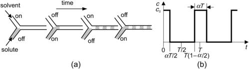
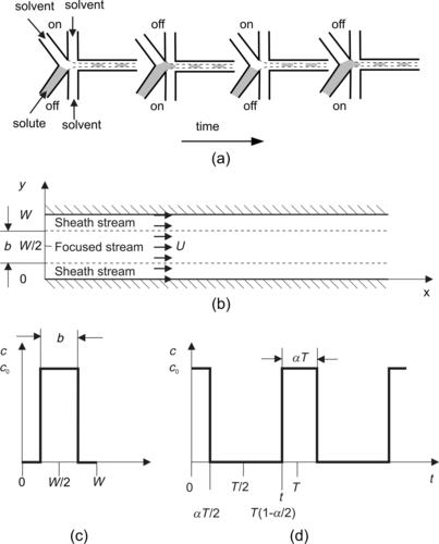
Sequential segmentation is a process where the solvent and the solute streams are broken up into segments along the axial direction. Because mixing occurs in the axial direction, the axial dispersion may lead to faster mixing. According to Section 2.3, the axial dispersion coefficient may be of several orders of magnitudes higher than pure molecular diffusion. Sequential segmentation is implemented by alternate switching of the inlet flows (Fig. 5.9 (a)) [28]. Switching is realized by two inlet valves or by controlling the pumps of the mixing liquids. The mixing ratio can be adjusted by the switching ratio (Fig. 5.9 (b)).
 |
| FIGURE 5.9 |
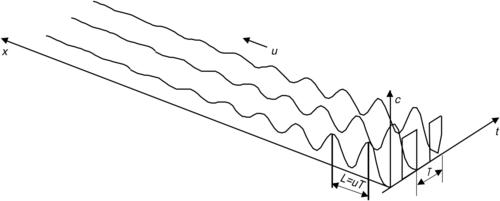
With a mean flow velocity of both fluids in the mixing channel and a switching period T, the characteristic mixing length is the segment length  (Fig. 5.10). The transport Eqn (2.22) can be reduced to the transient one-dimensional form [29]:
(5.16)
(5.17)
Normalizing the concentration by c0, the spacial variable by L, and the time by T results in the dimensionless form of (5.16):
(5.18)
(5.19)
Solving (5.18) with (5.19) and c∗ (∞)=α results in the transient concentration distribution (Fig. 5.10):
(5.20)
5.4. Segmentation Based on Injection
Segmentation based on injection introduces the solvent into the solute flow through a nozzle array. This concept also decreases the mixing path and increases the interfacial area between the solvent and the solute. Figure 5.11 shows a simple two-dimensional model of the concentration distribution around a single circular nozzle. The nozzle has a radius of R. The mass flow rate of the solute is  (kilograms per second), while the mass flow rate of the solvent is
  and an inlet concentration of c0. The solvent flow has a uniform velocity of and a concentration of c=0.
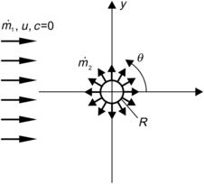
Considering a steady-state, two-dimensional problem and neglecting the source term, the transport equation reduces to the form
(5.21)
The general solution of (5.21) is the product of a velocity-dependent term and a symmetric term Γ:
(5.22)
Defining the variable  in the polar coordinate system as shown in Fig. 5.11, the boundary condition of the solute flow is, after Fick’s law:
(5.24)
(5.25)
Equation (5.23) can be rewritten for the polar coordinate system as
(5.26)
The solution of (5.26) is the modified Bessel function of the second kind and zero order:
(5.27)
The solution of (5.21) with the previously mentioned boundary conditions is
Introducing the Peclet number  , the dimensionless radial variable r∗=r/R, and the dimensionless concentration
(5.29)
the dimensionless form of (5.28) is
(5.30)
5.5. Focusing of Mixing Streams
5.5.1. Streams with the same viscosity
Hydrodynamic focusing reduces the mixing path by decreasing the width of the solute flow. Two solvent streams work as sheath flows in this concept (Fig. 5.13 (a)). Knight et al. [10] reported detailed experimental results of hydrodynamic focusing. However, the theoretical model reported in [10] was erroneous. The correct model is presented as follows:
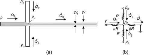
If the sheath streams have the same viscosity as the sample flow and all liquids are incompressible, the effect of hydrodynamic focusing can be represented by a simple network model. Assuming that the flow is laminar, the pressure difference across a microchannel is proportional to the flow rate. Figure 5.13 (b) shows the network model of hydrodynamic focusing where microchannels are represented by fluidic resistances. For simplicity, we further assume that both sheath microchannels have the same fluidic resistance of R, which is defined as the quotient between the applied pressure difference and the flow rate:  . The resistances of the inlet microchannel and the mixing microchannel are αR and βR, respectively. The factors α and β are determined by geometry parameters such as shape and size of channel cross-section as well as channel length. Taking the exit pressure as reference, the relations between the pressures at sample inlet, sheath flow inlets, and flow rates are given by the equation system:
(5.31)

(5.32)

The ratio between the sheath flow pressure and the sample pressure r = ps/p can be derived as follows:
(5.33)
The maximum and minimum values of the pressure ratio are subsequently determined by setting  and
and  , respectively:
(5.34)

(5.35)
The ratio  can be solved as an explicit function of α, β, and r from (5.32)
(5.36)
Example 5.1 (Network model for hydrodynamic focusing). The microchannel network depicted in Fig. 5.13 is made of silicon and glass by deep reactive ion etching and anodic bonding. The microchannel has a width of 100 μm and a height of 10 μm. The three inlet channels are 5 mm long, while the mixing channel is 20 mm long. What is the range of pressure ratio between the sheath flow and the sample flow? What is the required pressure ratio for a focusing width of 1 μm?
Solution. With a low aspect ratio h=H/W=0.1, the relation between the flow rate and the pressure derived in Example 2.3 can be used:
Thus, the fluidic resistance of the microchannel with a length L is
Because the cross-section of the microchannel network remains constant, the fluidic resistance is proportional to the channel length. From the geometry of the given channel network, we have

The maximum and minimum pressure ratios are

For a focusing width of Wf = 1 μm, we have
Solving the above linear equation results in the required pressure ratio for a focused width of 1 μm:
5.5.2. Streams with different viscosities
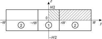
The following model analyzes the effect of hydrodynamic focusing for reducing the width of the mixing streams. In the model, the sample stream is sandwiched between two identical sheath streams (Fig. 5.14). The sample stream and the sheath stream are assumed to be immiscible. Figure 5.14 shows the geometry of the channel cross-section with the above two phases. The channel has a width 2W and a height H. The position of the interface is rW. Since the model is symmetrical regarding y-axis and z-axis, only one-fourth of the cross-section needs to be considered [11].
The velocity distribution u1 and u2 in the channel can be described by the Navier–Stokes equations:
(5.38)
(5.40)
The no-slip conditions at the wall are
The symmetry condition at the z∗-axis is
(5.42)
At the interface between the sample flow and the sheath flow, the velocity and the shear rate are continuous:
(5.43)
For a flat channel (h≪1), the position of the interface can be estimated as
(5.44)
(5.45)
5.5.3. Combination of hydrodynamic focusing and sequential segmentation
Both hydrodynamic focusing and sequential segmentation can be combined to improve convective/diffusive mixing in a microchannel [29]. The concept reduces mixing paths in both transversal and axial directions. Figure 5.16 describes this mixing concept. The micromixer has four inlets and one outlet. Two inlets are used for the sheath flows. The middle two inlets are used for sequential segmentation. The solvent and the solute are switched alternately so that segments of them are formed in the focused stream. The final mixing ratio is determined by both, the focusing ratio of the inlet flows and the switching ratio of the two focused flows.
 |
| FIGURE 5.16 |
The analytical model assumes a rectangular microchannel with width W and height H. For a microchannel with low aspect ratio (W≫H), the flow inside the microchannel is similar to that between two parallel plates. The model assumes a uniform velocity profile in the transversal direction (y-axis) and a pressure-driven velocity profile in the channel height (z-axis):
(5.46)
(5.47)
Figure 5.16 (a) shows the two-dimensional model of the mixing concept based on hydrodynamic focusing and sequential segmentation. Assuming that all the liquids involved in the system have the same viscosity, the velocity in the mixing channel is uniform across all streams. The focusing ratioβ=b/W can be adjusted by the flow rate ratio between the sheath streams and the focused streams. Considering the above effective diffusion coefficient in axial direction (5.47) and the molecular diffusion coefficient in transversal direction, the analytical model for combined hydrodynamic focusing and sequential segmentation in the domain depicted in Fig. 5.16 (a) can be described by a transient two-dimensional transport equation:
(5.48)
(5.49)
(5.50)
(5.51)
Normalizing spatial variables by the segment length , the time by the switching period T, and the concentration by the initial solute concentration c0:x∗=x/(UT), y∗=y/UT, W∗=W/UT, t∗=t/T, c∗=c/c0, the transport Eqn (5.48) has the dimensionless form:
(5.52)
(5.53)
(5.54)
(5.55)
(5.56)
The boundary conditions at the channel walls are
(5.57)
Using the method of separation of variables and the above conditions, the solution of (5.52) is
(5.58)
(5.59)
5.6. Gradient Generator Based on Diffusive Mixing
A well-defined concentration gradient is a reproduceable experimental platform to study the response of cells to molecular gradients, which is important for many pathological and physiological phenomena such as immune response, cancer metastasis, and stem cell differentiation. Gradient sensing is the main path leading to these phenomena. In living organisms, cells respond and migrate along gradients of biochemical cues. Microtechnology allows the design and implementation of platforms for the generation of concentration gradient with precise control over spatial and temporal resolution. The objective of designing a gradient generator is a well-defined concentration distribution and not a homogenous concentration field as in a micromixer. These platforms can mimic cellular environment. Drug screening and detailed investigations of disease processes can be carried out in a controlled manner.
The design of gradient generator follows the same principles of designing micromixers based on molecular diffusion. By controlling the diffusion/convection process in microchannels, a desired spatial and temporal concentration distribution can be achieved. Based on their working principles, gradient generators can be classified as parallel lamination and free-diffusion gradient generators.
Parallel lamination gradient generators provide a stable gradient and can be tuned quickly by flow control. However, the constant flow is not suitable for cells which do not adhere to the substrate. Even for cells that can adhere to the substrate, the shear stress caused by the flow does not represent the real physiological condition. For cell assays with parallel lamination gradient generator, special designs to minimize the shear stress should be considered.
Free-diffusion gradient generator can solve the problem with shear stress. However, the shapes of the concentration gradients are limited by the diffusion process. The gradient takes a long time to establish and is difficult to control dynamically.
5.6.1. Parallel lamination gradient generator
As analyzed in the previous sections, parallel lamination at high Peclet numbers can maintain the concentration of each stream due to the dominant convective transport. A desired concentration distribution can be designed by generating streams with a given concentration and subsequent laminating them with flow at high Peclet number. At a relatively low Peclet number, the concentration distribution is dominated by diffusion and can be predicted by a simple analytical model discussed in the previous sections on designing parallel lamination micromixers.
Jeon et al. proposed a pyramid design for a parallel lamination gradient generator (Fig. 5.18 (a)) [31]. The original three inlets at the top of the pyramid are split and recombine to form many branches. The solute and the solvent are mixed in the branches to form a given concentration. At the bottom of the pyramid, the branches are merged to form the desired concentration distribution. The microfluidic pyramid network was modeled as a resistive network with left-right symmetry. The network is modeled by connecting the horizontal channel with a resistance of RH and the vertical branches with a resistance of RV. The vertical branches are much longer than the connecting horizontal channels; thus their corresponding resistances are also much larger (RV>>RH). Due to the symmetry, the flow rate in each vertical branch is the same throughout the same order B. With the total number of branches B and the number of vertical branch v=0..B-1 (Fig. 5.18 (b)), the splitting ratios to the left and right at each junction are [31] and [32]
 |
| FIGURE 5.18 Parallel lamination gradient generator: (a) design concept and (b) branch number B and numbering vertical branches v. (Reprinted with permission from [32].) |
(5.60)

Similar to parallel lamination micromixer, the shape of the concentration distribution can be tuned by changing the flow rate ratio of the inlet streams at the top of the pyramid network. The larger the number of the inlet streams, the more shapes of the concentration distribution can be achieved. Dertinger et al. [32] extended the basic design of [31] to realize more complex concentration distributions. For a given number of inlets n, the concentration distribution of the gradient generator can empirically fit into a polynomial of (n – 1) order:
(5.61)
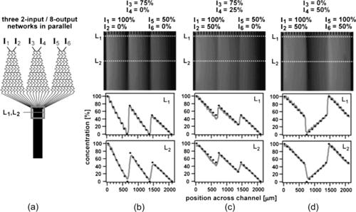
Thus, linear and parabolic concentration distributions can be generated with three inlets (Fig. 5.19). Repeating the same pyramid design and combining the streams in a single outlet can generate a periodic concentration gradient (Fig. 5.20). Using different solutes at the inlets leads to overlapping concentration gradient that potentially can be used for screening the combined effect of two or more solute types.
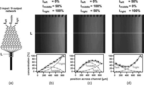 |
| FIGURE 5.19 Concentration distribution formed by a parallel lamination gradient generator: (a) a gradient forming network with three inlets and nine outlets; (b) linear gradient; and (c) and (d) parabolic gradient. (Reprinted with permission from [32].) |
 |
| FIGURE 5.20 (Reprinted with permission from [32].) |
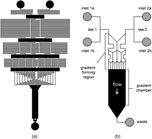
Campbell and Groisman [33] improved the above split-and-recombine concept with a premixing network. The device starts with two inlets, but the splitting junction has three outlets. The split-and-recombine network produces N outlets with different concentrations. The outlets then joined to form the desired concentration distribution. Unlike the previous designs of Jeon et al. [31] and Dertinger et al. [32], the vertical branches have different lengths, thus different resistance and different flow rates (Fig. 5.21 (a)). The different flow rates allow tailoring the amount of different concentrations, leading to a tunable concentration distribution.
 |
| FIGURE 5.21 |
Amarie et al. [34] used splitting junction with both two and three outlets. The gradient-generating mixing channels can be designed to be shorter and the overall split-and-recombine section is shorter than the previous designs which used serpentine design for the vertical mixing channels (Fig. 5.21 (b)). The shorter channel length and the shorter residence time allow faster switching between different concentration distributions. Since switching was mostly realized with external pumps, faster switching of the concentration distribution can be achieved with integrated microvalves [35].
5.6.2. Free-diffusion gradient generator
Free-diffusion gradient generator forms the concentration field in a no-flow environment such as microchannels with high fluidic resistance, porous membranes, or hydrogel. The concentration gradient is formed by diffusion of the molecules between a source and a sink. Because of the slow molecular diffusion process, free-diffusion gradient generators need a longer time to establish the concentration field as compared to parallel lamination gradient generator.
Saadi et al. [36] formed a one-dimensional concentration gradient in a ladder-like microchannel network. The source and sinks are two parallel microchannels, which are connected by an array of microchannels with a much smaller depth (Fig. 5.22 (a)). The high fluidic resistance of the microchannel array prevents the fluid to flow from the source to the sink and allows the gradient to build up based on pure molecular diffusion. This gradient generator was successfully used for neutrophil chemotaxis. Atencia et al. [37] developed a two-dimensional concentration gradient in a circular chamber with three access ports working as sources and sinks (Fig. 5.22 (b)). Switching the sources and sinks allow the formation of a dynamic concentration field. A time of about 15 minutes is needed to establish the concentration gradient in the chamber with a diameter of 1.5 mm.
 |
| FIGURE 5.22 |
Diao et al. [38] established the concentration gradient across a channel with porous nitrocellulose membrane as side walls. Parallel microchannels work as the source and the sink. The disadvantage of free-diffusion gradient generator is the fixed shape of the concentration distribution, which is determined by the geometry of the gradient chamber and the boundary condition given by the sources and sinks. Wu et al. solve this problem by using a fixed concentration field established in a hydrogel membrane. A concentration gradient with an arbitrary shape can be formed by running microchannels across the static concentration field in a given way. The porous hydrogel membrane is sandwiched between two PDMS parts (Fig. 5.23 (a)). The upper PDMS part contains the source and the sink, the lower PDMS contains the microchannels for the concentration gradient. The gradient is established in the hydrogel by molecular diffusion. The concentration in the microchannels of the lower PDMS parts came in equilibrium with the concentration of the hydrogel. Thus, the shape of the concentration distribution is determined by the shape of the microchannels (Fig. 5.23 (b,c)). The amount of molecules released at the source can be controlled by an applied pressure [39]. Controlling individual injection nozzles with integrated microvalves allows dynamic control of complex concentration distributions [40].
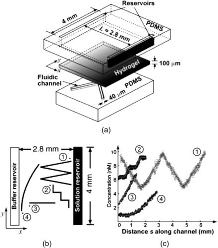 |
| FIGURE 5.23 Free-diffusion gradient generator with arbitrary shapes of concentration distribution: (a) design concept; (b) the shape of the microchannel; and (c) corresponding shape of the concentration gradient. (Reprinted with permission from [38].) |
To mimic the real cellular environment, the concentration should be generated in a three-dimensional matrix. The two-dimensional free-diffusion designs discussed above can be extended to three-dimensional designs by using gel matrices between the source and the sink.
References
[1] Kamholz, A.E.; Weigl, B.H.; Finlayson, B.A.; Yager, P., Quantitative analysis of molecular interaction in microfluidic channel: The T-Sensor, Anal. Chem. 71 (1999) 5340–5347.
[2] Ismagilov, R.F.; Stroock, A.D.; Kenis, P.J.A.; Whitesides, G.; Stone, H.A., Experimental and theoretical scaling laws for transverse diffusive broadening in two-phase laminar flows in microchannels, Appl. Phys. Lett. 76 (2000) 2376–2378.
[3] Kamholz, A.E.; Yager, P., Molecular diffusive scaling laws in pressure-driven microfluidic channels: deviation from one-dimensional Einstein approximations, Sens. Actuators B Chem. 82 (2002) 117–121.
[4] Hinsmann, P.; Frank, J.; Svasek, P.; Harasek, M.; Lendl, B., Design, simulation and application of a new micromixing device for time resolved infrared spectroscopy of chemical reactions in solutions, Lab Chip 1 (2001) 16–21.
[5] Hessel, V.; Hardt, S.; Loewe, H.; Schoenfeld, F., Laminar mixing in different interdigital micromixers: I. Experimental characterization, AIChE J. 49 (2003) 566–577.
[6] Hardt, S.; Schoenfeld, F., Laminar mixing in different interdigital micromixers: II. Numerical simulations, AIChE J. 49 (2003) 578–584.
[7] Haverkamp, V.; Ehrfeld, W.; Gebauer, K.; Hessel, V.; Loewe, H.; Richter, T.; Wille, C., The potential of micromixers for contacting of disperse liquid phases, Fresenius. J. Anal. Chem. 364 (1999) 617–624.
[8] Bessoth, F.G.; de Mello, A.J.; Manz, A., Microstructure for efficient continuous flow mixing, Anal. Commun. 36 (1999) 213–215.
[9] Kakuta, M.; et al., Micromixer-based time-resolved NMR: applications to ubiquitin protein conformation, Anal. Chem. 75 (2003) 956–960.
[10] Knight, J.B.; Vishwanath, A.P.; Brody, J.; Austin, R., Hydrodynamic focusing on a silicon chip: mixing nanoliters in microseconds, Phys. Rev. Lett. 80 (1998) 3863–3866.
[11] Wu, Z.; Nguyen, N.T., Rapid mixing using two-phase hydraulic focusing in microchannels, Biomed. Microdevices 7 (2005) 13–20.
[12] Jensen, K., Chemical kinetics: smaller, faster chemistry, Nature 393 (1998) 735–736.
[13] Walker, G.M.; Ozers, M.S.; Beebe, D.J., Cell infection within a microfluidic device using virus gradients, Sens. Actuators B Chem. 98 (2004) 347–355.
[14] Yi, M.; Bau, H.H., The kinematics of bend-induced mixing in micro-conduits, Int. J. Heat Fluid Flow 24 (2003) 645–656.
[15] Wong, S.H.; Ward, M.C.L.; Wharton, C.W., Micro T-mixer as a rapid mixing micromixer, Sens. Actuators B Chem. 100 (2004) 365–385.
[16] Lim, D.S.W.; Lim, D.S.W.; Shelby, J.P.; Kuo, J.S.; Chiu, D.T., Dynamic formation of ring-shaped patterns of colloidal particles in microfluidic systems, Appl. Phys. Lett. 83 (2003) 1145–1147.
[17] Wong, S.H.; Bryant, P.; Ward, M.; Wharton, C., Investigation of mixing in a cross-shaped micromixer with static mixing elements for reaction kinetics studies, Sens. Actuators B Chem. 95 (2003) 414–424.
[18] Gobby, D.; Angeli, P.; Gavriilidis, A., Mixing characteristics of T-type microfluidic mixers, J. Micromech. Microeng. 11 (2001) 126–132.
[19] Groisman, A.; Steinberg, V., Efficient mixing at low Reynolds number using polymer additives, Nature 410 (2001) 905–908.
[20] Gan, H.Y.; Lam, Y.C.; Nguyen, N.T.; Yang, C.; Tam, K.C., Efficient mixing of viscoelastic fluids in a microchannel at low Reynolds number, Microfluid Nanofluidics 3 (2006) 101–108.
[21] Schoenfeld, F.; Hessel, V.; Hofmann, C., An optimised split-and-recombine micro-mixer with uniform chaotic mixing, Lab Chip 4 (2004) 65–69.
[22] S. Wiggins and J.M. Ottino, Foundation of chaotic mixing, Phil. Trans. R. Soc. Lond. A, Vol. 362, pp. 937–970.
[23] Ottino, J.M.; Wiggins, S., Introduction: mixing in microfluidics, Phil. Trans. R. Soc. Lond. A 362 (2004) 923–935.
[24] Branebjerg, J.; Gravesen, P.K.P.; Nielsen, J.; Rye, C., Fast mixing by lamination, Proceedings of the IEEE Micro Electro Mechanical Systems (MEMS) (1996) 441–446.
[25] Schwesinger, N.; Frank, T.; Wurmus, H., A modular microfluid system with an integrated micromixer, J. Micromech. Microeng. 6 (1996) 99–102.
[26] Gray, B.L.; Jaeggi, D.; Mourlas, N.J.; Van Drieenhuizen, B.P.; Williams, K.R.; Maluf, N.I.; Kovacs, G.T.A., Novel interconnection technologies for integrated microfluidic systems, Sens. Actuators A Phys. 77 (1999) 57–65.
[27] He, B.; Burke, B.J.; Zhang, X.; Zhang, R.; Regnier, F.E., A picoliter-volume mixer for microfluidic analytical systems, Anal. Chem. 73 (2001) 1942–1947.
[28] Tan, C.K.L.; Tracey, M.C.; Davis, J.B.; Johnston, I.D., Continuously variable mixing-ratio micromixer with elastomer valves, J. Micromech. Microeng. 15 (2005) 1885–1893.
[29] Nguyen, N.T.; Huang, X.Y., Mixing in microchannels based on hydrodynamic focusing and time-interleaved segmentation: modelling and experiment, Lab Chip 5 (2005) 1320–1326.
[30] Nguyen, N.T.; Huang, X.Y., Modeling, fabrication and characterization of a polymeric micromixer based on sequential segmentation, Biomed. Microdevices J. 8 (2006) 133–139.
[31] Jeon, N.L.; Dertinger, S.K.W.; Chiu, D.T.; Choi, I.S.; Stroock, A.D.; Whitesides, G.M., Generation of solution and surface gradients using microfluidic systems, Langmuir 16 (2000) 8311–8316.
[32] Deringer, S.K.W.; Chiu, D.T.; Jeon, N.L.; Whitesides, G.M., Generation of gradients having complex shapes using microfluidic networks, Anal. Chem. 73 (2001) 1240–1246.
[33] Campbell, K.; Groisman, A., Generation of complex concentration profiles in microchannels in a logarithmically small number of steps, Lab Chip 7 (2007) 264–272.
[34] Amarie, D.; Glazier, J.A.; Jacobson, S.C., Compact microfluidic structures for generating spatial and temporal gradients, Anal. Chem. 79 (2007) 9471–9477.
[35] Irimia, D.; Liu, S.Y.; Tharp, W.G.; Samasani, A.; Toner, M.; Poznansky, M.C., Microfluidic system for measuring neutrophil migratory responses to fast switches of chemical gradients, Lab Chip 6 (2006) 191–198.
[36] Saadi, W.; Rhee, S.W.; Lin, F.; Vahidi, B.; Chung, B.G.; Jeon, N.L., Generation of stable concentration gradients in 2D and 3D environments using a microfluidic ladder chamber, Biomed. Microdevices 9 (2007) 627–635.
[37] Atencia, J.; Morrow, J.; Locascio, L.E., The microfluidic palette: a diffusive gradient generator with spatio-temporal control 9 (2009) 2707–2714.
[38] Diao, J.P.; Young, L.; Kim, S.; Fogarty, E.A.; Heilman, S.M.; Zhou, P.; Shuler, M.L.; Wu, M.M.; DeLisa, M.P., A three-channel microfluidic device for generating static linear gradients and its application to the quantitative analysis of bacterial chemotaxis, Lab Chip 9 (2009) 1797–1800.
[39] Wu, H.K.; Huang, B.; Zare, R.N., Generation of complex, static solution gradients in microfluidic channels, J. Am. Chem. Soc. 128 (2006) 4194–4195.
[40] Keenan, T.M.; Hsu, C.H.; Folch, A., Microfluidic "jets" for generating steady-state gradients of soluble molecules on open surfaces, Appl. Phys. Lett. 89 (2006) 114103.
[41] Chung, B.G.; Lin, F.; Jeon, N.L., A microfluidic multi-injector for gradient generation, Lab Chip 6 (2006) 764–768.
..................Content has been hidden....................
You can't read the all page of ebook, please click here login for view all page.