
Chapter 2. Fundamentals of mass transport in the microscale
Chapter Outline
2.1. Transport Phenomena10
2.2. Molecular Diffusion22
2.4. Chaotic Advection36
2.5. Viscoelastic effects53
2.6. Electrokinetic Effects55
2.7. Magnetic and Electromagnetic Effects66
2.8. Scaling Law and Fluid Flow in Microscale68
References71
Transport phenomena in micromixers can be described theoretically at two basic levels: molecular level and continuum level. The two different levels of description correspond to the typical length scale involved. Continuum model can describe most transport phenomena in micromixers with a length scale ranging from micrometers to centimeters. Most micromixers for practical applications are in this range of length scale. Molecular models involve transport phenomena in the range of one nanometer to one micrometer. Mixers with length scale in this range should be called “nanomixer.” The term “micromixer” in this book will cover devices with submillimeter length dimension.
2.1. Transport Phenomena
Transport phenomena in micromixers can be described theoretically at two basic levels: molecular level and continuum level. The two different levels of description correspond to the typical length scale involved. Continuum model can describe most transport phenomena in micromixers with a length scale ranging from micrometers to centimeters. Most micromixers for practical applications are in this range of length scale. Molecular models involve transport phenomena in the range of one nanometer to one micrometer. Mixers with length scale in this range should be called “nanomixer.” The term “micromixer” in this book will cover devices with submillimeter length dimension.
At the continuum level, the fluid is considered as a continuum. Fluid properties are defined continuously throughout the space. At this level, fluid properties, such as viscosity, density, and conductivity, are considered as material properties. Transport phenomena can be described by a set of conservation equations for mass, momentum, and energy. These equations of change are partial differential equations, which can be solved for physical fields in a micromixer, such as concentration, velocity, and temperature.
Miniaturization technologies have pushed the length scale of microdevices further. In the event of nanotechnology, scientists and engineers will encounter more phenomena at molecular level. At this level, transport phenomena can be described through molecular structure and intermolecular forces. Because many micromixers are used as microreactors, a fundamental understanding of molecular processes is important for designing devices with length scale in the micrometer to centimeter range.
2.1.1. Molecular level
At molecular level, the simplest description of transport phenomena is based on the kinetic theory of diluted monatomic gases, which is also called the Chapman–Enskog theory. The interaction between nonpolar molecules is represented by the Lennard–Jones potential, which has an empirical form of:
(2.1)
| Boltzmann constant: kB=1.38×10⁻²³J/K, dij=cij=1. | ||
| Gas | Characteristic Energy (ɛ/kB) | Characteristic Diameter σ (nm) |
|---|---|---|
| Air | 97.0 | 0.362 |
| N2 | 91.5 | 0.368 |
| CO2 | 190.0 | 0.400 |
| O2 | 113.0 | 0.343 |
| Ar | 124.0 | 0.342 |
(2.2)
The Lennard–Jones model results in the characteristic time:
(2.3)
(2.4)
Example 2.1 (Estimation of gas viscosity using kinetic theory). Estimate the viscosity of pure nitrogen at 25 °C.
Solution. Using the Lennard–Jones parameters of nitrogen listed in Table 2.1, the dimensionless temperature is:
(2.5)
(2.6)
(2.7)
Kinetic theory can be applied to liquids as well. In this model, the motion of liquid molecules is confined within a space limited by its neighboring molecules. Based on this theory, the viscosity of a liquid can be estimated as:
(2.8)
The models of viscosity for gas (2.4) and for liquid (2.8) show opposite temperature dependency. While the viscosity of gases increases with higher temperature, the viscosity of liquids decreases.
Example 2.2 (Dynamic viscosity of water). If the molar volume of water at 25°C is 18×10−6m3/mol, determine the viscosity of water at this temperature.
Solution. The boiling temperature of water under atmospheric pressure is assumed to be 100°C. According to (2.8), the viscosity of water can be estimated as:
In the previous discussion, continuum properties are derived from the molecular model using statistic methods. If there are not enough molecules for good statistics, numerical tools are used for modeling transport phenomena at the molecular level. There are two numerical methods: molecular dynamics (MD) and direct simulation Monte Carlo (DSMC). While MD is a deterministic method, DSMC is a statistical method.
Molecular dynamics is a numerical method for modeling the motion of single molecules. The interactions between the molecules can be described by the classical second law of Newton. The simplest model of a molecule is a hard sphere of a mass m. The binary interaction between two molecules is determined by the Lennard–Jones force (2.2):
(2.9)
(2.10)
Because of its deterministic nature, MD is extremely expensive in terms of computational resources. Less resources would be needed if the system is modeled with a statistic method.
Direct simulation Monte Carlo is a statistic method for modeling at the molecular level. In DSMC, many molecules are modeled as a single particle. The interactions between the molecules of each particle are determined statistically, while the motion of the particle is modeled deterministically. The basic steps of DSMC are [3]:
• Determination of particle motion,
• Indication and cross-referencing of particles,
• Simulation of particle collision, and
• Sampling of macroscopic properties.
2.1.2. Continuum level
At continuum level, transport phenomena are described with a set of conservation equation. Because flow in micromixers is laminar, we do not need to deal with turbulent flow, which is impossible to solve analytically. The three basic conservation equations are:
• Conservation of mass: continuity equation,
• Conservation of momentum: Newton’s second law or Navier–Stokes equation, and
• Conservation of energy: first law of thermodynamics or energy equation.
Solving these three equations will result in three basic variables: the velocity field v, the pressure field p, and the temperature field T. Fluid properties, depending on the thermodynamic state (pressure p and temperature T), such as density, viscosity, thermal conductivity, and enthalpy, can be derived from these variables and fed back into the conservation equations. The above three equations are formulated for a single phase of homogenous composition. In micromixers, most fluids carry one or more species other than the carrying fluids. If the mixers are used as microreactors, chemical reactions also need to be considered. Thus, in addition to the above three conservation equations, two further equations are needed to describe the transport of species in micromixers:
• Conservation of species: convective/diffusive equation and
• Laws of chemical reactions.
2.1.2.1. Conservation of mass
The continuity equation has the general form:
(2.12)
2.1.2.2. Conservation of momentum
Conservation of momentum is described by Newton’s second law:
(2.13)
(2.14)
(2.15)
 |
| FIGURE 2.2 Cross section of channels considered in Table 2.2: (a) circle; (b) ellipse; (c) concentric annulus; and (d) rectangle. |
| Channel Type | Solution |
|---|---|
| Circle |  |
| Ellipse |  |
| Concentric annulus |  |
| Rectangle |  |
 |
| FIGURE 2.3 Distribution of dimensionless velocity according to Table 2.2 (y∗=y/a, z∗=z/a): (a) circle; (b) ellipse (a=2b); (c) concentric annulus (a=2b); and (d) rectangle (a=2b). |
Many micromachining technologies result in microchannels with a rectangular cross section. The following examples investigate the flows of a single phase as well as multiple phases in rectangular microchannels.
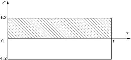
Example 2.3 (Single-phase flow in a rectangular microchannel). A liquid flow in a rectangular microchannel of width W and height H. The viscosity of the liquid is μ. Determine the velocity distribution in this microchannel and the flow rate if a pressure difference of Δp is applied across the channel length of L.
Solution. The fully developed flow in the microchannel is governed by Navier–Stokes equations:
(2.16)
 |
| FIGURE 2.4 |
(2.17)
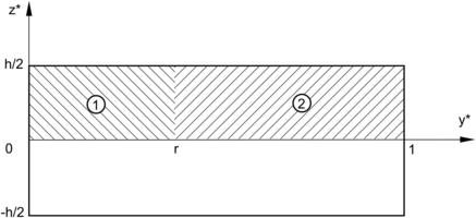
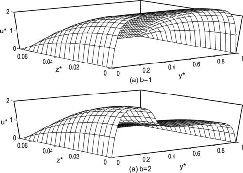
Example 2.4 (Velocity distribution of streams with different viscosities in a rectangular microchannel). Two immiscible fluids flow side by side in a rectangular microchannel of width W and height H. The viscosity ratio and flow rate ratio of the two fluids are β=μ2/μ1 and  , respectively. Determine the velocity distribution in this microchannel [4].
Solution. The fully developed flow in the microchannel is governed by Navier–Stokes equations:
 |
| FIGURE 2.5 |
Figure 2.6 shows the typical velocity distribution in a rectangular channel for streams with different flow rates. For streams with the same viscosity, the velocity distribution is flat.
2.1.2.3. Conservation of energy
The conservation of energy is governed by the first law of thermodynamics:
(2.18)
(2.19)
(2.20)
(2.21)
2.1.2.4. Conservation of species
The conservation of species leads to the diffusion/convection equation:
(2.22)
2.2. Molecular Diffusion
2.2.1. Random walk and Brownian motion
A random walk is the path traced by a particle taking successive steps, each in a random direction. The construction of a simple random walk follows the three basic rules:
• The particle starts at a predefined point,
• The distance done by each step is equal, and
• The direction from one point to the next is random.
Following these rules, random walk of a particle can be realized with a simple program. Considering a one-dimensional random walk on a line, the particle has a random choice of two directions for each of its steps. The distance done by each step is assumed to be s. The position x(n) at a step (n) can be described as
(2.23)
(2.24)

Jan Ingenhousz, a Dutch doctor, was the first to observe the irregular motion of coal dust particles on the surface of alcohol in 1785 [5]. However, the botanist Robert Brown, who observed, in 1827, pollen particles floating in water under the microscope [6], is credited for the discovery of this motion. The Brownian motion of particles in a liquid is due to the instantaneous imbalance in the force exerted by the small liquid molecules on the particle. Thus, the diffusion coefficient of this particle can be derived from the force balance equation.
2.2.2. Stokes–Einstein model of diffusion
The time evolution of the position of the Brownian particle itself can be described approximately by the force balance equation where the random force of the liquid molecules represents one term in the balance. This equation is called the Langevin equation:
(2.25)
(2.26)
(2.27)
(2.28)
(2.29)
(2.30)
(2.31)
(2.32)
(2.33)
2.2.3. Diffusion coefficient
2.2.3.1. Diffusion coefficient in gases
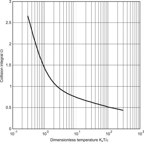
Using the kinetic theory discussed in Section 2.1.1, diffusion coefficient in meters squared per second between two gases i and j can be formulated as [7]:
(2.34)
(2.35)
(2.36)
Example 2.5 (Estimation of diffusion coefficient of gases). Estimate the diffusion coefficient of hydrogen in air at 282K. Lennard–Jones potential parameters of air and hydrogen are (σ1=0.3711nm,  and (σ2=0.2827nm,
  , respectively. The molecular weights of air and hydrogen are 29 and 2 respectively. The experimental value is 0.710×10⁻⁴m2/sec.
Solution. Although air consists mainly of oxygen and nitrogen, we assume air as a gas molecule. According to (2.35), the collision diameter between air and hydrogen is:
According to (2.36), the dimensionless temperature is:
According to Fig. 2.1, the collision potential is approximately 0.88. Thus, the diffusion coefficient of hydrogen in air at 282K is:
The estimated diffusion coefficient is 33% lower than the measured data.
2.2.3.2. Diffusion coefficient in liquids
While diffusion coefficients of gases are on the order of 10−5m2/sec, diffusion coefficients of liquids are on the order of 10−9m2/sec. The diffusion coefficients of large molecules can be on the order of 10−11m2/sec. Diffusion coefficient of a molecule i in a solute j with a viscosity μj can be estimated by the Stokes–Einstein equation:
(2.37)
(2.38)
Example 2.6 (Diffusion coefficient of a large molecule in water). Fibrinogen is a protein that plays a key role in blood clotting. Fibrinogen significantly increases the risk of stroke. This protein molecule has a rod shape of 67nm in length and 2.2nm in diameter. Estimate the diffusion coefficient of fibrinogen in water at 25°C. Dynamic viscosity of water at this temperature is μ=0.903×10⁻³Pa·s.
Solution. The large molecule can be assumed to have the ellipsoid shape with a=67×10−9m and b=2.2×10⁻⁹nm. According to (2.38), the characteristic diameter of a fibrinogen molecule is:
(2.39)
Thus, based on the Stokes–Einstein equation (2.37), the diffusion coefficient of fibrinogen is:
The diffusion of a large molecule in water is about six orders slower than that of gases.
2.2.3.3. Diffusion coefficient of electrolytes
Salts and many other molecules dissolve in water to form cations and anions. However, they do not diffuse as a single molecule, because different ions have different diffusion coefficients. Table 2.3 and Table 2.4 show the diffusion coefficients of typical cations and anions in water at 25°C. However, both anion and cation together should have the same diffusion coefficient to maintain the charge neutrality. It is interesting to observe from Table 2.3 that the diffusion coefficient of proton H+ is about five times larger than other ions. Since the size difference between H+ and the other ion is not significant, H+ should have a different diffusion mechanism in water. H+ actually does not move through water but reacts with a water molecule and releases a proton on the other side. This new proton can cause another reaction. This chain reaction speeds up the transport process and leads to a much higher diffusion coefficient of H+ in water [7].
| H+ | Li+ | Na+ | K+ | Rb+ | Cs+ | Ag+ | NH4+ | Ca2+ | Mg2+ | La3+ |
|---|---|---|---|---|---|---|---|---|---|---|
| 9.31 | 1.03 | 1.33 | 1.96 | 2.07 | 2.06 | 1.65 | 1.96 | 0.79 | 0.71 | 0.62 |
| OH− | F– | Cl– | Br– | I– | NO3+ | CH3COO– | B(C6H5)4– | ||
|---|---|---|---|---|---|---|---|---|---|
| 5.28 | 1.47 | 2.03 | 2.08 | 2.05 | 1.90 | 1.09 | 0.53 | 1.06 | 0.92 |
The diffusion coefficient of a molecule consisting of a cation of charge z1 and an anion of charge z2 is:
(2.40)
Example 2.7 (Diffusion coefficient of sodium chloride). Determine the diffusion coefficient of sodium chloride at 25°C.
Solution. From Table 2.3 and Table 2.4, the diffusion coefficients of sodium cation and chloride anion are D1=1.33×10⁻⁹m2/sec and D2=2.03×10⁻⁹m2/sec, respectively. Applying z1=+1 and z2=−1 in (2.40) results in the diffusion coefficient of sodium chloride:
The diffusion coefficients of electrolytes in water are about four orders smaller than those of gases and about two orders larger than those of large molecules.
In many lab-on-a-chip applications, micromixers are needed for mixing proteins. The behavior of proteins is very complex. A protein molecule consists of chains of amino acids. The molecular weight is very large and can be on the order of 105. A protein molecule has a large number of side chains that end in amino (–NH2) or carboxylic acid (–COOH) groups. Depending on the pH concentration, amino groups can be positively charged to become ( ) and carboxylic acid groups become negatively charged (–COO−). Therefore, the net charge of a protein can be either positive or negative. Further, depending on the pH, the protein chains can be folded differently, resulting in various sizes and shapes. The different charges and shapes make the diffusion coefficient of proteins depend on the pH concentration. Furthermore, the diffusion coefficient of protein also depends strongly on its concentration and the concentration of electrolytes, such as NaCl.
Many solute molecules, such as surfactant, also have diffusion coefficients that depend on the solute concentration. At high concentrations, the molecules can aggregate to form micelles. The aggregation and the electrostatic interaction cause the strong concentration dependence of the diffusion coefficient.
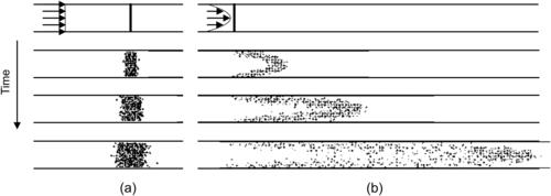
2.3. Taylor Dispersion
Taylor dispersion is an effective mechanism for mixing a solute in a distributed velocity field, such as a pressure-driven flow in a microchannel. This axial effect arises from a coupling between molecular diffusion in the transverse direction and transverse distribution of the flow velocity. Figure 2.8 illustrates the difference between molecular diffusion in a plug-like flow and Taylor dispersion in a distributed flow. In a uniform flow field, such as the plug-like electroosmotic flow, advection and diffusion are independent. Axial diffusion is the same as molecular diffusion (Fig. 2.8 (a)). In a distributed flow field, such as the pressure-driven flow with a parabolic velocity distribution, the solvent is stretched more in the middle of the channel than near the wall, due to axial convective transport. The resulting concentration gradient between the different fluid layers is then blurred by diffusion in the transverse direction (see Fig. 2.8 (b)). As a result, the solute appears to be “diffusing” in the axial direction at a rate that is much faster than what would be predicted by ordinary molecular diffusion.
 |
| FIGURE 2.8 |
2.3.1. Two-dimensional analysis
The dispersion coefficients are derived by a two-dimensional model, involving one axial and one transversal spatial dimension. G. I. Taylor was the first to present a working model for the transverse average that managed to capture the influences of both transverse diffusion and the transverse variations of the fluid velocity field. The analysis of Taylor [10] is based on the model of a long cylindrical capillary with a radius r0 (Fig. 2.9). The derivation of the dispersion coefficient given below follows Brenner and Edwards [11]. According to Table 2.2, the velocity distribution in the capillary cross section is:
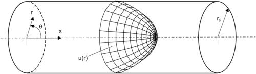
(2.41)
(2.42)
(2.43)
The boundary and initial conditions of (2.42) are:
(2.44)

If the observer moves along the flow with the mean velocity  , we can consider a new axial coordinate x∗:
(2.46)
Next, an average specie concentration is introduced:
(2.47)
(2.48)
(2.49)
(2.50)
(2.51)
In order to introduce the dispersion coefficient or the so-called effective diffusion coefficient D∗, the conservation of species (2.46) is written in the flux form as:
(2.52)
(2.53)
(2.55)
(2.56)
(2.57)
The specie conservation equation can be now formulated as:
(2.58)
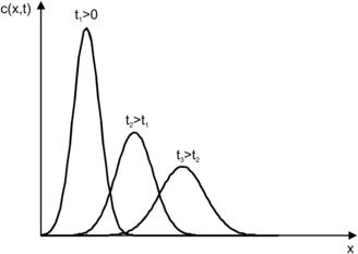
The above partial differential equation can be solved analytically. For instance, if the initial condition of the specie concentration is a pulse  , where δ(x) is the Dirac function, the transient one-dimensional solution of the average concentration is:
(2.59)
Figure 2.10 shows the typical concentration distribution of the one-dimensional dispersion at different time instances.
 |
| FIGURE 2.10 |
A few years after Taylor’s publication, Aris provided a firmer theoretical framework for this theory by using a moment analysis [12]. He also generalized the problem to handle time-periodic flows [13]. Following the works of Taylor and Aris, there are several other contributions to the theory of deriving effective transport models for the transverse averages of solutes flowing through channels with more general cross-sectional geometries and flow properties. Common techniques are the use of asymptotic analysis [14], [15], [16] and [17], the theory of projection operators [18], the center manifold theory [19]. All the above works only dealt with nonreactive problems. Johns and DeGance considered the influences of a system of linear reactions upon Taylor dispersion [20]. Yamanaka and Inui used their projection operator theory to solve problems involving a single irreversible reaction [21]. The following example by Bloechle [22] demonstrates an intuitive approach similar to that of Taylor [10]. The approach is called the mean-fluctuation method commonly used in turbulent flow.
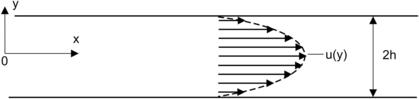
Example 2.8 (Taylor dispersion in Poiseuille flow between two parallel plates[22]). Determine the dispersion coefficient of a Poiseuille flow between two parallel plates with a gap of 2h as depicted in Fig. 2.11.
 |
| FIGURE 2.11 |
Solution. Because of the symmetric geometry, only half of the model is considered (−∞<x<∞, 0<y<h). The governing Eqn (2.22) reduces to the two-dimensional form of the parallel plates model (t>0):
(2.60)
(2.61)
The concentration and velocity can be formulated as the sum of an average component and a fluctuating component:
(2.63)
Averaging (2.63) from 0 to h leads to:
(2.64)
The initial condition of the above equation is:
(2.65)
Similar to Taylor’s original approach, the dispersion coefficient can be derived from the above equation if the fluctuation concentration c′ is known. Subtracting (2.64) from (2.63) leads to the partial differential equation for c′:
(2.66)
(2.67)
(2.69)
(2.70)
(2.71)
(2.72)
(2.73)
(2.74)
The final expression for the fluctuating component of the concentration is:
(2.76)
(2.77)
2.3.2. Three-dimensional analysis
For axisymmetric channel geometry, such as a cylindrical capillary, the two-dimensional analysis described in the above subsection is appropriate. For real channel geometry, the cross-sectional velocity profile and, consequently, the dispersion coefficient also depend on the channel shape. In other words, the second transversal spatial dimension needs to be considered in the analysis.
Dutta et al. [23] introduce a factor f into (2.77) to consider the three-dimensional effect of Taylor dispersion:
(2.78)
 |
| FIGURE 2.12 (after [23]) |
Because of the velocity gradient at the sharp corners of a rectangular channel, factor f increases from f=1.76 in the case of a square channel cross section (d/W=1) to f=7.95 in the case of a shallow channel (W≫d). The factor of an elliptical channel cross section can be calculated explicitly as:
Ajdari et al. [24] argued that for a shallow channel W≫d with a continually varying height, the dispersion coefficient is not determined by the channel height and aspect ratio. The channel width W is the only geometric parameter that determines the dispersion coefficient. For instance, the dispersion coefficients for channels with triangle, parabolic, and elliptical cross sections are:
(2.80)
(2.81)
(2.82)
In the case of an elliptical cross section, a low aspect ratio W≫d refers to an eccentricity of unity ɛ=1. Substituting ɛ=1 in (2.79) results in a factor:
2.4. Chaotic Advection
2.4.1. Basic terminologies
The term chaotic advection refers to the phenomenon where a simple Eulerian velocity field leads to a chaotic response in the distribution of a Lagrangian marker, such as a tracing particle [25]. Advection refers to species transport by the flow. A flow field can be chaotic even in the laminar flow regime. Chaotic advection can be created in a simple two-dimensional flow with time-dependent disturbance or in a three-dimensional flow even without time-dependent disturbance. It is to be noted that chaotic advection is not turbulent. For a flow system without disturbance, the velocity components of chaotic advection at any point in space remain constant over time, while the velocity components of turbulence are random. The streamlines of the steady chaotic advection flow across each other, causing the particles to change their paths. Under chaotic advection, the particles diverge exponentially and enhance the mixing between the solvent and solute flows. In a time-periodic system, the condition for chaos is that streamlines cross at two consecutive time instants.
There are few terminologies related to visualization of an Eulerian velocity field. The first and most common terminology is the pathline, also called trajectory of a fluid particle in the flow field. In experiments, pathlines, orbits, or trajectories can be obtained by an image with a long-time exposure of a fluorescent fluid particle.
If the particles are idealized so that they are small enough not to disturb the flow and large enough so that molecular diffusion is neglected, they can move passively with the flow. The particle transport mechanism can simply be described by the advection equations:
(2.85)

Mathematically, pathlines or trajectories can be obtained by solving (2.85) with the initial condition at t=0 (x=x0, y=y0, z=z0). Numerical integration methods, such as the Runge–Kutta method, can be used for determining the positions of the particles.
In a two-dimensional flow, streamlines are given by the solution of:
(2.86)
(2.87)
A streakline through a point (x, y, z) at a time instance τ is the curve formed by all particles, which (t<τ) passed through this point previously. In experiments, the streakline is the tracing curve of a nondiffusive tracer injected into the flow at the given point.
Example 2.9 (Trajectories and streamlines). An Eulerian velocity field is given as:
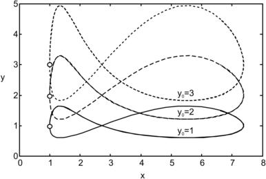
All variables and constants are dimensionless. Determine the trajectories and streamlines of particles initially at (x0=1, y0=1), (x0=1, y0=2), and (x0=1, y0=3).
Solution. Solving the differential equations with the initial condition (x0, y0) results in the position of the fluid particle as a function of time:
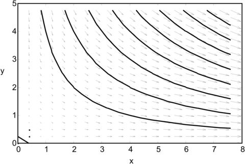
Figure 2.13 shows graphically the above pathlines, with the three initial particle positions, a=1, b=2, and c=π/2.
 |
| FIGURE 2.13 |
The stream function  can be solved for the explicit form using the equation system (2.87). Taking the time t as constant, u(x, y, t)=x sin(at), and v(x, y, t)=y sin(bt+c), we have:
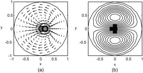
It is apparent that streamlines are time dependent. Figure 2.14 shows the streamlines as the level sets of stream function  .
.
Equation (2.85) represents a system of coupled ordinary differential equations (ODEs). Similar dynamical systems in engineering and physics have shown a strong chaotic behavior. Poiseuille flow in a straight microchannel is considered as a one-dimensional incompressible flow at low Reynolds number. The dynamics of this flow is simple and nonchaotic. In the case of a two-dimensional flow, the dynamic behavior of the flow is more interesting. The two-dimensional continuity equation:
(2.88)
The terminologies for chaotic advection can be borrowed from the more established field of dynamical systems theory. The advection equations (2.85) can be solved explicitly for the fluid particle position (x, y, z) at a given time t. The solution of (x, y, z) is then used for describing the motion of fluid particles in a region R, such as a channel cross section, and thus can be called a mapping function S[26]. From an initial condition (t=0), R can be transformed into a new region using S. This transformation or mapping can mathematically be described as S(R). Each transformation is called an advection cycle, which corresponds to a mixing element in different micromixer designs such as sequential lamination, discussed later in this book. Repeating these mixing elements n times refers to repeated application of S to R, or Sn(R). With the discrete number of advection cycles, the transformation S is understood as a discrete, not continuous, operation as in the case of the time function.
If the fluid is assumed to be incompressible, then the volume (in a three-dimensional case) or the area (in a two-dimensional case) are preserved after each transformation. Thus, the above mapping function S is called a volume-preserving transformation or a area-preserving transformation.
A trajectory of a point after applying many discrete transformations is called an orbit. If a point p returns to the same place after N transformations, the orbit is periodic with a period of N. The two typical periodic orbits are the stable elliptic orbit and the unstable hyperbolic orbit. Elliptic orbits lead to a region that does not mix with the surrounding fluid and thus are bad for mixing. Hyperbolic orbits lead to squeezing and stretching of fluid regions and thus are good for mixing. In an unstable orbit, if the fluid particle changes its path at the intersection of the same orbit, the orbit is called homoclinic. If the fluid particle changes its path at the intersection with another orbit, the orbit is called heteroclinic.
The trajectories of a chaotic three-dimensional flow are complicated. Three-dimensional positions of fluid particles can be reduced into a two-dimensional map called the Poincaré section. In a time-periodic system, Poincaré section is a collection of intersections of trajectories with a plane. The continuous trajectories become discrete points of the transformations Pn→Pn+1. The time needed between the two points Pn and Pn+1 does not need to be the period of the system. In three-dimensional space-periodic systems, the plane is taken at the same position of the repeated spatial structure. A trajectory intersects all these periodic planes at several points. The collection of these points forms the Poincaré section. In this case, the transformation Pn→Pn+1 is the advection cycle.
2.4.2. Examples of chaotic advection
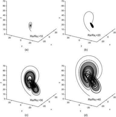
2.4.2.1. Lorentz’s convection flow
For a three-dimensional system, the equations in (2.85) are more than enough to create a nonintegrable or chaotic dynamics. Lorenz [27] derived a simplified system of equations for convection rolls in the atmosphere:
(2.89)
2.4.2.2. Dean flow in curved pipes
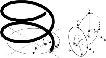
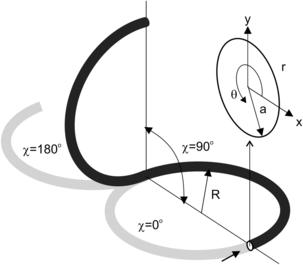
The flow field inside a curved pipe was first derived by Dean [28]. For a more detailed review on flow in curved pipes, see [29]. The following detailed derivation was given by Gratton [30]. The model for the flow in a toroidal pipe is depicted in Fig. 2.16. The pipe has the form of a toroid of a radius of R. The pipe diameter is a. The coordinate system for this model is based on the cylindrical coordinate, where s is the coordinate of the toroid’s center line q. The metric of this coordinate system is:

(2.90)
(2.92)
(2.93)
(2.94)
(2.95)
(2.97)
(2.98)
(2.99)
(2.100)
(2.101)
(2.102)
(2.103)
(2.104)
For the s component, all the ɛ terms are canceled from the expression of u in (2.104). The functions of h(r) and h′(r) are:
(2.106)
Further normalization of the time and s by Reɛ/144 and Reɛ/288 results in the dimensionless velocity components:
(2.107)
(2.108)
 |
| FIGURE 2.18 |
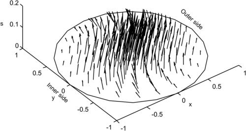
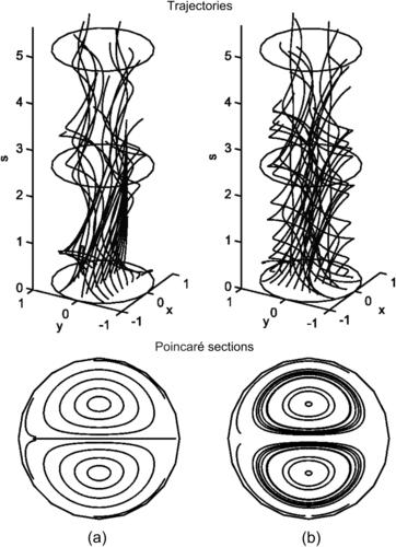
The trajectories of the fluid particles are calculated using the velocity solutions (2.107) and numerical integration with the Runge–Kutta method. Projecting the particle position on a single two-dimensional cross section results in the Poincaré section. Figure 2.19 shows the trajectories and Poincaré sections of the Dean flow where the s-axis is straightened for clarity. The results clearly show that independent of the orientation seeding lines, the Poincaré sections follow the streamlines as depicted in Fig. 2.18 (b). If this flow is used in a micromixer, the solvent and solute should be introduced on the left and right of the cross section or the outer and inner side of the curved channel (Fig. 2.18), so that the trajectories of the fluid particle can sample both sides of the channel. If the solvent and solute are introduced in the upper and lower halves of the channel, the trajectories will keep them in their respective channel section and advective mixing will not work. Even if the solvent and solute enter at the outer and inner side of the curved channel, the trajectories are stable, elliptic, and homoclinic. Transversal transport is advective but not chaotic. This means, they do not cross each other. Therefore, chaotic advection cannot be realized with the original Dean flow.
 |
| FIGURE 2.19 |
The above analysis assumes a small ratio between the pipe diameter and radius of curvature, a/R≪1. For realistic channel designs, this ratio can be approximately unity, and the secondary flows are more obvious. In this case, the flow is characterized by the Dean number:
(2.109)
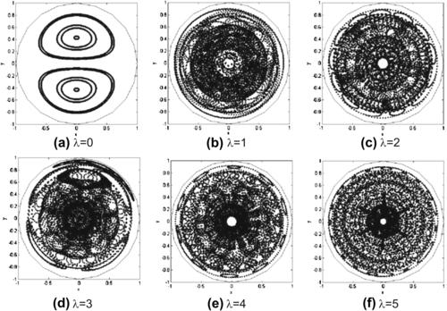
2.4.2.3. Flow in helical pipes [32]
In helical pipes, the cross section rotates around the pipe center line q (Fig. 2.20). Assuming a constant torsion of τ, the rotation at s is τs. Further, a constant curvature k=dΦ/ds is assumed. Based on this assumption, Germano [31] derived the metric:
The flow in this coordinate system has only a second-order dependence on τ. Thus, the solution (2.107) can be used for helical pipes by changing the basis to the new coordinate system (2.110). The solution for the velocity field is then:
(2.111)
(2.113)
 |
| FIGURE 2.21 |
The Poincaré sections of flow helical pipes with different geometry parameters are shown in Fig. 2.22. The flow is initially sampled with a seeding line parallel to the y-axis. At λ=0, there is no torsion and the pipe is a torus. The flow is clearly not chaotic; the particles follow the streamlines. At λ>0, chaotic advection is apparent.
2.4.2.4. Flow in twisted pipes [32]
While a straight channel is one dimensional, a three-dimensional flow (transverse cross-sectional plane and longitudinal axis) can be created in curved channels. In such curved channels, secondary vortices in the transverse cross-sectional plane can move fluid particles between the center of the channel and its wall. A unit of the simplest configuration for chaotic advection is depicted in Fig. 2.23. The secondary flow in a twisted pipe causes the so-called Dean vortices. Fluid particles rotate with an angle of χ between successive units. The following analysis was reported by Jones et al. [32].
Using the polar coordinate system (θ, r) in the transverse x – y plane, the stream function and the axial velocity u are determined through the following dimensionless equation system:
(2.114)

(2.115)
The first-order perturbation solution results in the following equations of the particle motion [32]:
(2.116)
Using the angle θ to describe the three-dimensional motion of fluid particles, the velocity components in x – y plane can be formulated as [32]:
(2.117)
(2.118)
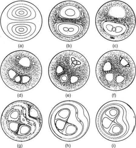 |
| FIGURE 2.24 Poincaré sections of twisted pipes with different twisting angles χ (α/β=100): (a) χ=0; (b) χ=π/16; (c) χ=π/8; (d) χ=π/4; (e) χ=3π/8; (f) χ=π/2; (g) χ=5π/8; (h) χ=3π/4; (i) χ=7π/8. (Reproduced from [32] by permission of Cambridge University Press.) |
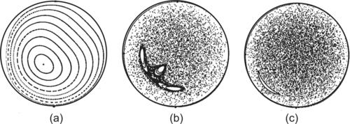 |
| FIGURE 2.25 Poincaré sections of twisted pipes with different twisting angles χ (α/β=200): (a) χ=π/4; (b) χ=π/2; (c) χ=3π/4. (Reproduced from [32] by permission of Cambridge University Press.) |
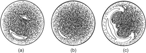 |
| FIGURE 2.26 Poincaré sections of twisted pipes with different ratios α/β (χ=π/2): (a) α/β=50; (b) α/β=150; (c) α/β=250. (Reproduced from [32] by permission of Cambridge University Press.) |
2.4.2.5. Flow in a droplet
With the increasing popularity of droplet-based microfluidics, mixing in droplets becomes a crucial task in designing a droplet-based lab-on-a-chip. The analytical solution for the internal flow inside a droplet was first reported by Hadamard [33]. Consider a spherical microdroplet with a radius a. The droplet experiences a uniform shear flow of a velocity in the z-axis. We now consider the viscosity ratio β=μ1/μ2, where μ1 is the viscosity of the droplet fluid and μ2 is the viscosity of the surrounding fluid. Normalizing the spatial variables by the droplet radius a, the velocity by and the time by  result in the dimensionless equations of particle motion inside the droplet [34]:
The flow described by (2.119) is actually one dimensional and not chaotic because it has two invariants [35]:
(2.120)
(2.121)
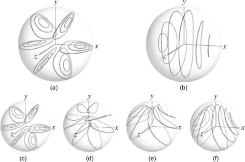 |
| FIGURE 2.27 Streamlines of flow inside a spherical droplet; the flow direction of the surrounding fluid is in z-axis: (a) external uniform flow; (b) external shear flow; (c) superposition flow with α=0, β=1; (d) superposition flow with α=0.2, β=1; (e) superposition flow with α=0.4, β=1; and (f) superposition flow with α=0.6, β=1. (Reprinted with permission from [34].) |
2.5. Viscoelastic effects
In most analysis and design considerations of micromixers, the solute and solvent are assumed to be Newtonian fluids. In these fluids, the viscosities do not depend on the velocity gradient or the shear stress. This means at a given temperature and pressure, the viscosity is a constant and the velocity gradient is linearly proportional to the shear stress. The Newtonian assumption is true for solvents and solutes with small molecules. However, if they contain large molecules such as long polymers, the viscosity is also a function of the shear stress. Since the shear stress and viscosity gradient in microscale increase with miniaturization, nonlinear effects can be expected and exploited for mixing applications.
At the molecular level, viscoelastic fluids can be described by two models: network model and single-molecule model [2]. The network model is based on the formation and rupture of junctions between polymer molecules. The network model is suitable for solutions with high polymer concentration. Dilute solutions are better described with a single-molecule model where interactions between the molecules are not frequent. The polymer molecule is represented by a “dumb-bell” or “bead-string” model where two spheres are connected by a spring. Kinetic theory with Stokes drag theory and Brownian motion can be used with this model for deriving macroscopic properties.
Fluids with large molecules display elastic behavior due to the stretching and coiling of the polymer chain. Here, these fluids and their behaviors are called viscoelastic fluids and viscoelastic effects respectively. The most apparent viscoelastic effect is the change of velocity profile in a channel. The dimensionless velocity profile of a viscoelastic fluid in a circular capillary can be approximated as [2]:
(2.122)
The next viscoelastic effect, which is relevant to mixing in microscale, is the entry flow at a contraction. The operation point of a viscoelastic flow is represented by the Wi–Re diagram, where Wi is the Weissenberg number and Re is the Reynolds number. With a characteristic length scale Lc, the mean velocity , the density ρ, and the zero-stress viscosity μ0, the Reynolds number is defined here as:
(2.123)
(2.124)
The characteristic residence time is the inverse value of the characteristic shear rate  and is defined as:
(2.125)
(2.126)

2.6. Electrokinetic Effects
2.6.1. Electroosmosis
Electrokinetic effects are based on an electric double layer at the interface between a solid and a liquid or between two liquids. This double layer is also called the Debye layer. This section focuses on the interface between a solid and a liquid. In general, there are four basic electrokinetic effects:
• Electroosmosis is the flow of a liquid in an electric field relative to a stationary charged surface.
• Electrophoresis is the motion of a charged particle in an electric field relative to the surrounding liquid.
• Streaming potential is the opposite effect of electroosmosis. An electric potential is created when a liquid is forced to flow relative to a charged surface.
• Sedimentation potential is the opposite effect of electrophoresis. An electric potential is created when charged particles are forced to flow relative to a surrounding liquid.
2.6.1.1. The Debye layer
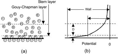
The Debye layer is an electric double layer, which occurs due to interaction between an electrolyte and a charged solid surface. Ions in an electrolyte solution are attracted to the charged surface and form a thin charge layer, which is called the Stern layer. The Stern layer is attracted to the surface due to the electrostatic force. The layer leads to the formation of a thicker charge layer in the solution. This diffuse and mobile layer is called the Gouy–Chapman layer. The Stern layer and the Gouy–Chapman layer together form the Debye layer (Fig. 2.29 (a)). Because the Gouy–Chapman layer is mobile, it can move if an electric field is applied. The interface between the Stern layer and the Gouy–Chapman layer is called the shear surface. The potential of the charged solid surface is called the wall potential Ψwall. The potential of the shear surface is called the zeta potential (Fig. 2.29 (b)). The potential distribution in the electrolyte solution can be described by the one-dimensional Poisson equation:
 |
| FIGURE 2.29 |
(2.127)
(2.128)
(2.129)
The charge density ρel in a symmetric electrolyte is proportional to the concentration difference between cations and anions:
(2.131)
(2.132)
(2.133)
(2.134)
2.6.1.2. Electroosmotic transport effect
The continuum models using mass and energy conservation equations can be used for describing the electroosmotic transport effects. The conservation of momentum needs to consider the electrostatic force created by the electric field:
(2.135)
(2.136)
(2.137)

With a constant viscosity μ and a constant zeta potential  , the electroosmotic velocity is proportional to the electric field strength Eel. The negative sign shows that the flow direction is opposite to the field direction. The proportional factor is called the electroosmotic mobility:
Equation (2.137) shows that the analysis of electrokinetic flows in a microchannel network can be replaced by the analysis of a resistance network. Electric currents and potentials can be calculated based on the basic Kirchhoff law:
• The sum of all currents at a node is zero,
• The sum of all voltages in a closed loop is zero.
After determining the potentials at the nodes of the network, the field strengths in each microchannel can be calculated. The velocity can then be determined by the given electroosmotic mobility.
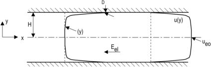
2.6.1.3. Electrokinetic flow between two parallel plates
Figure 2.31 shows the model of electrokinetic flow between two parallel plates. The velocity distribution U(y) of an electrokinetic flow between two parallel plates can be derived from the Navier–Stokes equation. For further simplicity, the variable U(y) is introduced:
(2.140)

(2.141)
(2.143)
(2.144)
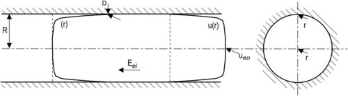
2.6.1.4. Electrokinetic flow in a cylindrical capillary
Figure 2.32 shows the model of electrokinetic flow in a cylindrical capillary. The Navier–Stokes equation and the Poisson–Boltzmann equation are formulated for the cylindrical coordinate system:
(2.147)
(2.148)
(2.149)
(2.150)
(2.151)
(2.152)
(2.153)
(2.154)
(2.155)
(2.156)
(2.157)
(2.158)
2.6.1.5. Electrokinetic flow in a rectangular microchannel
Due to the characteristics of microtechnology, many micromixers have a rectangular cross section. Figure 2.33 shows the model of electrokinetic flow in a rectangular microchannel. The Navier–Stokes equation and the Poisson–Boltzmann equation are formulated in the Cartesian coordinate system as:

(2.159)
Following dimensionless variables are introduced:
(2.160)
(2.161)
(2.162)
(2.163)
(2.164)


2.6.1.6. Ohmic model for electrolyte solutions
In this section, a model for electrolyte solutions is derived. This model is useful for formulating mixing problems in an electrokinetic system. The model was formulated by Chen et al. [37], who followed the approach of Levich [38]. We consider here a monovalent binary electrolyte (|z+|=|z−|=1), where the subscripts + and − denote the cation and anion, respectively. The local charge density and conductivity σel are determined as:
(2.165)
(2.166)
The conservation of species can be formulated for the ions as:
(2.168)
(2.169)
(2.170)
(2.171)
(2.172)
(2.173)
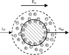
2.6.2. Electrophoresis
Electrophoresis is the motion of a charged particle relative to the surrounding liquid in an electric field (Fig. 2.34). Because of the small size and low Reynolds number involved, the Stokes model can be assumed for the motion of the particle:
(2.174)
(2.175)
(2.177)
(2.178)
(2.179)
(2.180)
(2.181)
2.6.3. Dielectrophoresis
Dielectrophoresis (DEP) is the motion of a dielectric particle in a dielectric fluid. Because the particle is charge neutral, dielectric force is caused by the inhomogeneity of the electric field. Assuming a homogenous linear dielectric fluid with a susceptibility of χ, the polarization field P of the fluid is given as:
(2.182)
The displacement field D of the fluid is:
(2.183)
(2.184)
The dielectric force acting on a dipole moment in an inhomogeneous electric field is:
(2.185)
For a spherical particle with the permittivity ɛp, the polarization leads to a dipole moment m:
(2.186)
2.7. Magnetic and Electromagnetic Effects
2.7.1. Magnetic effects
Although magnetic forces are body forces and therefore do not scale favorably in micromixers, high field gradients can be achieved with integrated microcoils. The use of liquids with magnetic properties and an external actuating magnetic field promises to be a niche for inducing transversal transport and chaotic advection in micromixers. The best candidate for this concept is ferrofluid. Pure substances such as liquid oxygen also behave like a magnetic liquid or ferrofluid. However, the term ferrofluid is commonly referred to as colloidal ferrofluid. The magnetic property of this fluid is credited to ferromagnetic nanoparticles, usually magnetite, hematite, or some other compounds containing iron 2+ or 3+. These nanoparticles are solid, single-domain magnetic particles that are suspended in a carrier fluid. The particles are coated with a monolayer of surfactant molecules to avoid them to stick to each other. Because the size of the particles is on the order of nanometers, Brownian motion, which represents the kinetic or thermal energy of the particles, is able to disperse them homogenously in the carrier fluid. The dispersion is strong enough that the solid particles do not agglomerate or separate even under strong magnetic fields. A typical ferrofluid is opaque to visible light. It is to be noted that the term magnetorheological fluid (MRF) refers to liquids similar in structure to ferrofluids but differing in behavior. MRF particle sizes are on the order of micrometers that are one to three orders of magnitude larger than those of ferrofluids. MRF also has a higher volume fraction on the order of 20–40%. Exposing MRF to a magnetic field can transform it from a light viscous fluid to a thick solid-like material [39].
Ferromagnetic nanoparticles are fabricated based on size reduction through ball milling, chemical precipitation, and thermophilic iron reducing bacteria. In ball milling, magnetic material of several micrometers in size such as magnetite powder is mixed with carrier liquid and surfactant. The ball milling process takes approximately 1000h. Subsequently, the product mixture undergoes centrifuge separation to filter out oversize particles. The purified mixture can be concentrated or diluted in the final ferrofluid.
Synthesis by chemical precipitation is a more common approach in which the particles precipitate out of solution during chemical processes. A typical reaction for magnetite precipitation is:
(2.187)
The reaction product is subsequently coprecipitated with concentrated ammonium hydroxide NH4OH. Next, a peptization process transfers the particles from water-based phase to an organic phase, such as kerosene with a surfactant, for example, oleic acid. The oil-based ferrofluid can then be separated by a magnetic field.
Another approach for fabrication of ferrofluid is based upon thermophilic bacteria that reduce amorphous iron oxyhydroxides to nanometer-sized iron oxides. The thermophilic bacteria are able to reduce a number of different metal ions. Thus, this approach allows incorporating other compounds, such as Mn(II), Co(II), Ni(III), Cr(III)), into magnetite. Varying the composition of the nanoparticles can adjust magnetic, electrical, and physical properties of the substituted magnetite and consequently of the ferrofluid. Ferromagnetic particle with extremely low Curie temperature can be designed with this method. Most of the particle materials commonly used in ferrofluid have much higher Curie temperatures. The temperature dependence of magnetic properties can be used for micromixing applications.
At the typical channel size of microfluidics (about 100μm), ferrofluid flow in a microchannel can be described as a continuum flow. The governing equations are based on the conservation of mass and conservation of momentum. In the case of temperature-dependent magnetic properties, the conservation of energy may be needed for calculating the temperature field. The Navier–Stokes equation for a ferrofluid has the following form:
(2.188)
(2.189)
The first term in (2.189) shows that the magnetic force is a body force, which is proportional to the volume. According to the scaling law, or the so-called cube-square law, magnetic force will be dominated by viscous force in microscale. However, the second term in (2.189) may have advantages in microscale due to the high-magnetic-field gradient that is achievable with integrated microcoils. As mentioned previously, ferrofluid with low Curie temperature is readily available. Magnetization can be controlled by adjusting the temperature from room temperature to an acceptably low Curie temperature. The temperature dependence of magnetization can be implemented in the first term of (2.189); the magnetic force then has the form [40]:
(2.190)
2.7.1.1. Electromagnetic effects
Electromagnetic effect or magnetohydrodynamics (MHD) deals with behavior of electrically conducting fluids in a magnetic field. A magnetic field induces currents in a moving conductive fluid. A current passing through a conductive fluid can create forces on the fluid and affect the magnetic field. Similar to electrokinetics, MHD effects represent multiphysics problems, which require the coupling of the different fields. MHD effects can be described by the Navier–Stokes equations of fluid dynamics and Maxwell’s equations of electromagnetism.
The Navier–Stokes equation of an MHD flow has the form:
(2.191)
(2.192)
2.8. Scaling Law and Fluid Flow in Microscale
The diffusion coefficient D, kinematic viscosity v, and the thermal diffusivity α=kpc – where k, p, and c are thermal conductivity, density, and specific heat, respectively – are transport properties and all have the same unit of m2/s. The ratios between these properties represent a group of nondimensional numbers that are characteristic for the interplay between the competing transport processes. These nondimensional numbers help to compare molecular diffusion with other transport processes in microfluidics.
The Schmidt number is the ratio between momentum transport and diffusive mass transport:
(2.193)
For most liquids and gases, the Schmidt number is larger than unity Sc≥1. This means in most cases spreading fluid motion is easier than molecules of the species.
Lewis number is the ratio between heat transport and diffusive mass transport:
(2.194)
The ratio between advective transport and momentum transport is called the Reynolds number:
(2.195)
Peclet number is the ratio between advective mass transport and diffusive mass transport:
(2.196)
The average diffusion time t over the characteristic mixing length Lmixing, also called the striation thickness, is represented by the Fourier number [7]:
(2.197)
(2.198)
Thus, the ratio between the channel length and channel width is:
(2.199)
If the inlets are split and rejoined as n pairs of solute/solvent streams, the mixing length is reduced to Lmixing=W/n. The ratio of the required channel length and channel width then becomes:
(2.200)
If the inlets are stretched and folded in n cycles, the mixing length is reduced to Lmixing=W/bn. The base b depends on the type of mixer. In the case of sequential lamination as discussed in the next section, the base is, for instance, b=2. The base could have a different value in the case of mixing based on chaotic advection. The ratio between the required channel length and the channel width is:
(2.201)
In general, fast mixing can be achieved with smaller mixing path and larger interfacial area. If the channel geometry is very small, the fluid molecules collide most often with the channel wall and not with other molecules. In this case, the diffusion process is called Knudsen diffusion [7]. The ratio between the distance of molecules and the channel size is characterized by the dimensionless Knudsen number:
(2.202)
(2.203)
Among the above dimensionless numbers, Reynolds number Re represents the flow behavior in the microchannel, while Peclet number (Pe) represents the ratio between advection and diffusion. Thus, these two numbers are suitable for characterizing the operation point of a micromixer. From the definitions (2.195) and (2.196), the relation between Pe and Re is:
(2.204)
In micromixers, the process of mixing and chemical reaction are related. Initially, mixing occurs first and is then followed by the chemical reaction. Subsequently, both mixing and chemical reaction occur in parallel. The ratio between the characteristic mixing time tmixing and reaction time treaction is called the Damköhler number:
(2.205)
References
[1] Hirschfelder, J.C.; Gurtiss, J.C.; Bird, R.M., Molecular Theory of Gases and Liquids. (1954) Wiley, New York.
[2] Bird, R.B.; Stewart, W.E.; Lightfoot, E.N., Transport Phenomena. second ed (2001) Wiley, New York.
[3] Garcia, A.L., Numerical Methods for Physics. second ed (2000) Prentice Hall, Englewood Cliffs.
[4] Wu, Z.; Nguyen, N.T., Convective-diffusive transport in parallel lamination micromixers, Microfluidics and Nanofluidics 1 (2004) 208–217.
[5] Bown, W., Brownian motion sparks renewed debate, New Scientist 133 (1992) 25.
[6] R. Brown, A brief account of microscopical observations made in the months of June, July and August, 1827, on the Particles contained in the pollen of plants; and on the general existence of active molecules in organic and inorganic bodies, Philosophy Magazine (4) 161–173, 1828.
[7] Cussler, E.L., Diffusion: Mass Transfer in Fluid Systems. second ed (1997) Cambridge University Press.
[8] Tayor, G.I., Diffusion by continuous movements, Proceedings of the London Mathematical Society vol. A20 (1921) 196.
[9] Einstein, A., Investigation on the Theory of Brownian Movement. (1956) Dover, New, York.
[10] Taylor, G.I., Dispersion of soluble matter in solvent flowing slowly through a tube, Proceedings of the Royal Society A 219 (1953) 186–203.
[11] Brenner, H.; Edwards, D.A., Macrotransport Processes. (1993) Butterworth-Heinemann, Boston.
[12] Aris, R., On the dispersion of a solute in a fluid flowing through a tube, Proceedings of the Royal Society A 235 (1956) 67–77.
[13] Aris, R., On the dispersion of a solute in a pulsating flow through a tube, Proceedings of the Royal Society A 259 (1960) 370–376.
[14] Fife, P., Singular perturbation problems whose degenerate forms have many solutions, Applicable Analysis 1 (1972) 331–358.
[15] Fife, P.; Nicholes, K., Dispersion in flow through small tubes, Proceedings of the Royal Society A 344 (1975) 131–145.
[16] Gill, W.N., A note on the solution of transient dispersion problems, Proceedings of the Royal Society A 298 (1967) 335–339.
[17] Gill, W.N.; Sankarasubramanian, R., A note on the solution of transient dispersion problems, Proceedings of the Royal Society A 316 (1970) 341–350.
[18] Yamanaka, T., Projection operator theoretical approach to unsteady convective diffusion phenomena, Journal of Chemical Engineering of Japan 16 (1983) 29–35.
[19] Watt, S.D.; Roberts, A.J., The accurate dynamic modelling of contaminant dispersion in channels, SIAM Journal of Applied Mathematics 55 (1995) 1016–1038.
[20] Johns, L.E.; Degance, A.E., Dispersion approximations to the multicomponent convective diffusion equation for chemically active systems, Chemical Engineering Science 30 (1975) 1065–1067.
[21] Yamanaka, T.; Inui, S., Taylor dispersion models involving nonlinear irreversible reactions, Journal of Chemical Engineering of Japan 27 (1994) 434–435.
[22] Bloechle, B.W., On Taylor Dispersion of Reactive Solutes in a Parallel-Plate Fracture-Matrix Syste. PhD Thesis (2001) University of Colorado.
[23] Dutta, D.; Ramachandran, A.; Leighton Jr., D.T., Effect of channel geometry on solute dispersion in pressure-driven microfluidic systems, Microfluidics and Nanofluidics 2 (2006) 275–290.
[24] Ajdari, A.; Bontoux, N.; Stone, H.A., Hydrodynamic dispersion in shallow microchannels: the effect of cross-section shape, Analytical Chemistry 78 (2006) 387–392.
[25] Aref, H., Stirring by chaotic advection, Journal of Fluid Mechanics 143 (1984) 1–21.
[26] Wiggins, S.; Ottino, J.M., Foundations of chaotic mixing, Proceedings of the Royal Society A 362 (2004) 937–970.
[27] Lorenz, E.N., Deterministic nonperiodic flow, Journal of the Atmospheric Sciences 20 (1963) 130–141.
[28] Dean, W.R., Note on the motion of a fluid in a curved pipe, Philosophy Magazine 4 (1927) 208–223.
[29] Berger, S.A.; Talbot, L.; Yao, L.S., Flow in curved pipes, Annual Reviews of Fluid Mechanics 15 (1983) 461–512.
[30] Gratton, M.B., The Effects of Torsion on Anomalous Diffusion in Helical Pipe. Thesis (2002) Department of Mathematics, Harvey Mudd College.
[31] Germano, M., On the effect of torsion on helical pipe flow, Journal of Fluid Mechanics 203 (1982) 1–8.
[32] Jones, S.W.; Thomas, O.M.; Aref, H., Chaotic advection by laminar flow in a twisted pipe, Journal of Fluid Mechanics 209 (1989) 335–367.
[33] Hadamard, J., Movement permanent lent D’une sphere liquide et visqueuse dans un liquide visqueux, Comptes Rendus 152 (1911) 1735.
[34] Stone, Z.B.; Stone, H.A., Imaging and quantifying mixing in a model droplet micromixer, Physics of Fluids 17 (2005) 1–11.
[35] Grigoriev, R.O.; Schatz, M.F.; Sharma, V., Chaotic mixing in microdroplets, Lab Chip 6 (2006) 1369–1372.
[36] Rodd, L.E.; Scott, T.P.; Boger, D.V.; Copper-White, J.J.; McKinley, G.H., The inertio-elastic planar entry flow of low-viscosity elastic fluids in micro-fabricated geometries, Journal of Non-Newtonian Fluid Mechanics 129 (2005) 1–22.
[37] Chen, C.H.; Lin, H.; Lele, S.K.; Santiago, J.G., Convective and absolute electrokinetic instability with conductivity gradients, Journal of Fluid Mechanics 524 (2005) 263–303.
[38] Levich, V.G., Physicochemical Hydrodynamics. (1962) Prentice-Hall, Englewood Cliffs.
[39] Rosenzweig, R.E., Ferrohydrodynamics. (1985) Cambridge University Press, Cambridge.
[40] Love, L.J.; Jansen, J.F.; McKnight, T.E.; Roh, Y.; Phelps, T.J., A magnetocaloric pump for microfluidic applications, IEEE Transactions on Nanobioscience 3 (2004) 101–110.
..................Content has been hidden....................
You can't read the all page of ebook, please click here login for view all page.