Definition. This function returns the logical value (Boolean value) FALSE.
Arguments. None
Background. This function is seldom used, because you can just enter the word false. Excel interprets the result returned by the function as a logical value (in this case, FALSE). The interpretation forced by numeric operations is the number value 0. You can check this by entering the formula =3+FALSE in a cell.
However, if you compare two cells, and one cell contains FALSE and the other cell 0, the result is FALSE.
You can enter false (which is not case-sensitive) directly in a worksheet or formula. Excel recognizes this word as the logical value FALSE and formats the cell accordingly. To avoid this, do one of the following:
Format the cell as text before you enter false (use Cells/Format/Format Cells on the Home tab in Excel 2007 and Excel 2010 and Format/Cells in earlier versions).
Enter a space before the word false.
Prefix the text with an apostrophe (‘).
Excel recognizes FALSE as a logical value even if you don’t enter the parentheses. This is different from other functions; for example, an error is generated if the function TODAY() is entered without the parentheses.
Logical values can be useful when you are evaluating expressions using the logical operators AND and OR:
The OR operator for two logical values is always TRUE unless both logical values are FALSE.
The AND operator for two logical values is always FALSE unless both logical values are TRUE.
Example. If you are working with conditional formats in one or more cells, the conditions can get complex, and using logical values can help to maintain clarity.
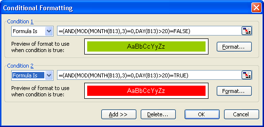
For example, you might want to highlight the days at the end of a quarter. These can be defined as the days after the twentieth day in the months of March, June, September, and December. If you use the TODAY() function to enter the current date into cell B13 of your worksheet, the formula
AND(MOD(MONTH(B13),3)=0;DAY(B13)>20
defines the days that you want to highlight. If this function is true, format the background color as red; if the value is false, format the background green. The formula
MOD(MONTH(B13),3)=0
determines whether the month is the last month of a quarter—in other words, whether the month number is exactly divisible by 3. The formula
DAY(B13)>20
is TRUE if the number of the day is greater than 20. Therefore,
=(AND(MOD(MONTH(B13),3)=0;DAY(B13)>20)=TRUE)
selects the last days in each quarter, and
=(AND(MOD(MONTH(B13),3)=0,DAY(B13)>20)=FALSE)
returns the remaining days.
To enter the formulas, click New Rule in the Styles/Conditional Formatting menu on the Home tab, and select Use A Formula To Determine Which Cells To Format. In the dialog box that appears, you can change the existing rules (see Figure 9-1).

In earlier Excel versions, select the Format/Conditional Formatting option to access the Conditional Formatting dialog box (see Figure 9-2).