
Syntax. ADDRESS(row_num,column_num,Abs,a1,sheet_text)
Definition. This function converts arguments into a text cell reference.
Arguments
row_num and column_num (required). The coordinates of the address. These arguments can be any expression that can be evaluated to a number that will create a valid reference (values from 1 through 65,536 for row_num and from 1 through 256 for column_num in Excel 2003 and earlier, and a maximum of 1,048,476 for row_num and 16,384 for column_num in Excel 2007 and Excel 2010).
Abs (optional). Indicates whether a reference is absolute or relative. Table 10-2 lists the valid arguments. The default value is 1.
Table 10-2. Reference Style Numbers
Reference Style | Abs Argument |
|---|---|
Absolute row and column | 1 |
Relative column, absolute row | 2 |
Relative row, absolute column | 3 |
Relative row and column | 4 |
a1 (optional). A logical value specifying the reference style: a1 = 1 or TRUE; R1C1 = 0 or FALSE. If the argument is omitted, a1 is used as the default.
sheet_text (optional). Puts a worksheet name and an exclamation point in front of the reference. The argument requires an expression that can be converted into text. If the argument is omitted, a simple cell reference is generated.
Background. You can use this function to generate the address of a cell in a worksheet. If the evaluation of the row_num and column_num arguments results in a positive fraction greater than 1, this value is truncated to the integer by removing the decimal places.
Addresses that include a sheet name do not verify that the sheet name exists.
Important
You cannot immediately use the result of the ADDRESS() function as a cell reference, because the result returned is a string. You can check this with the ISREF() function or by trying to add the string to a formula as a reference. The second example that follows shows how this problem can be solved.
Examples. The following examples show how this function is used.
Automatic Labels. Assume that you want to automatically label the columns in a table section that starts in column C with the letters A, B, and so on. You enter the formula
=LEFT(ADDRESS(1,COLUMN()-COLUMN($C$14)+1,4),1)
in the upper-left cell of the section and copy this formula into the columns to the right.
The COLUMN() function calculates the column number of the cell containing the formula. (The $C$14 argument in cell C14 doesn’t generate a circular reference.) Subtract the column values and add 1 to ensure that A is always the starting point. If you add 2, the starting point is B, and so on. The LEFT() function with the second argument of 1 returns a single character.
Indirect Addressing. The formula =ADDRESS(6,2) returns $B$6 as a string. To use the content of cell B6 in other calculations, use the INDIRECT() function to convert the argument into a valid reference. The formula
=INDIRECT(ADDRESS(6,2))
returns the content of cell B6.
Find the Last Cell in a Range. Sometimes you might have to use the content of the last cell in a list (or in a range) without knowing how long the list is.
Assume that you have a list containing deposits and payments (see Figure 10-1).
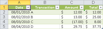
To use the account balance (here $37.75) at a different position in the worksheet or in a different worksheet, you enter a formula:
=INDIRECT(ADDRESS(COUNT(A:A)+1,4))
or
=INDIRECT(ADDRESS(COUNT(payments!A:A)+1,4,,,"payments"))
The COUNT() function calculates the number of the numeric values in column A (column A should contain only date values). You add 1 to take the title row into account, and the INDIRECT() function does everything else (as explained in the previous example).
The second formula assumes that the Payments worksheet contains your list (you pass this parameter to the ADDRESS() function).