
Syntax (Array Version). INDEX(array,row_num,column_num)
Syntax (Reference Version). INDEX(reference,row_num,column_num,area_num)
Definition. This function uses a row and/or column index to select one or more values from an array (multiple connected cells or expressions separated by a semicolon and enclosed in braces) or from a reference (which can contain one or more references to rectangular areas) based on index entries.
Arguments (Array Version)
array (required). Must be a range of cells or an array constant.
row_num (optional). Can be omitted if the array argument includes only one cell. This argument must evaluate to a positive integer and specifies the number of the row that holds the values to work with.
column_num (optional). An expression that must evaluate to a positive integer. This argument specifies the number of the column that holds the values to choose and can be omitted if the array reference consists of only a single column.
Arguments (Reference Version)
reference (required). Must evaluate to a reference to one or more cell ranges.
row_num and column_num (optional). Same as for the array version, but these arguments indicate the number of the row or column that holds the values to choose, and therefore they don’t have to evaluate to positive integers.
If the reference argument consists of multiple parts, these parts are numbered in the order in which they are entered.
area_num (optional). Selects a range specified in the reference argument pertaining to the order in which the ranges are defined.
Note
If the reference argument consists of only a single subarea, the area_num argument can be omitted. In this case, the reference version is identical to the array version.
Background. In the array version, the row_num and column_num arguments usually range from 1 through the number of rows or columns in the range or in a value list. If the range consists of only a single row (column), the row_num (column_num) argument can be omitted. To omit the row_num argument, enter two commas. If you omit several rows, you can reference the column specified in column_num with an array formula in the vertical cells. The same applies if you want to omit several columns.
If the row_num and column_num arguments exceed the range, you will get the #REF! error. The formula
=INDEX(B4:C6,3,2)
returns the element in C6 (third row, second column in the range B4:C6). Similarly, consider the following:
=INDEX({2;4;6;8},2,1)(This isn’t an array formula, so you have to enter the braces instead of pressing Ctrl+Shift+Enter.) The argument {2;4;6;8} is recognized as column, and the formula returns 4 (the second row in the column).
Array constants that include multiple columns constitute a special situation, because rows are separated by semicolons, and columns are separated by commas. For example, {11,12,13;21,22,23} is recognized as
|
|
|
|
|
|
The formula
=INDEX({11,12,13;21,22,23},2,3)returns 23 (second row, third column).
You can use the INDEX() function in an array formula as shown in the following example. If you enter
{=INDEX({11,12,13;21,22,23},0,3)}or
{=INDEX({11,12,13;21,22,23},,3)}as array formula in two vertical cells, the formula returns 13, 23. If you enter
{=INDEX({11,12,13;21,22,23},2,0)}or
{=INDEX({11,12,13;21,22,23},2)}as array formula in three horizontal cells, the formula returns 21, 22, 23. If the destination range is larger than the source range, the extra cells show the #N/A error.
In the reference version, the first argument must be a reference. If you want to use multiple ranges, each range must consist of contiguous cells. The reference argument for multiple references separated by semicolons must be enclosed in parentheses to ensure that Excel assigns the arguments correctly.
The order of the references in the argument is indicated by an integer, starting at 1, to identify the cell range in the area_num argument. The row_num and column_num arguments behave as in the array version.
If one of the row_num, column_num or area_num arguments exceeds the range, the function returns the #REF! error. The formula
=INDEX((B18:C20,E18:G19),3,2,1)
returns the reference to the element in the third row in the second column in the first range (C20).
INDEX() accepts named ranges in the reference argument. If you enter the name first for range B18:C20 (by selecting Defined Names/Define Name on the Formulas tab in Excel 2007 or Excel 2010 or Insert/Names/Define in earlier versions) and the name second for range E18 through G19, the formula
=INDEX((first,second),2,1,2)
returns a reference to the cell in the second row in the first column of the range named second: E19. You can also name all of the cells B18:C20,E18:G19 (in this order) with the name both. Then the formula
=INDEX(both,2,3,2)
returns the information in the third column in the second row of the second subarea: G19. You can omit the row_num or column_num argument or both (leaving the space between the commas empty) to reference columns or rows or an entire range. In this case, you have to use the formula as array formula or you will get the #VALUE! error unless the range consists of only one row or column.
Note
The row_num, column_num, and area_num arguments expect integers. If you pass decimal numbers, these numbers will not be rounded but truncated, and the decimal places will be removed.
Examples. The following examples show how this function is used.
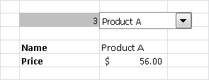
Searching Lists. This example demonstrates the array version of the function. Assume that you have a product list with the product names in column 1 and the prices in column 2. You maintain this list on a special worksheet (or the information is imported from a database). On a different worksheet, you want to use a combo box (a form control) to access and select the product names as well as write the price into a cell.
Name the columns PriceList and Products.
Insert a combo box, and specify the value Product as the input range and $B$28 as the cell range.
In any cell, enter
=INDEX(PriceList,B28,1)to display the product name.
In another cell, enter
=INDEX(PriceList,B28,2)to display the associated price. Figure 10-3 shows an example.
Note
You can also create a combo box from the control toolbox (ActiveX Control on the Developer tab in Excel 2007 or Excel 2010). Unlike a form control, which displays the index of the entry in the linked cell, the combo box control displays the text of the entry in the linked cell.
Finding Information. This example demonstrates the reference version of the function. Assume that you have divided an advanced training course into three parts and offer single-unit or complete conference reservations. You also offer an early-bird discount for participants who book before a deadline. The details are shown in Figure 10-4.
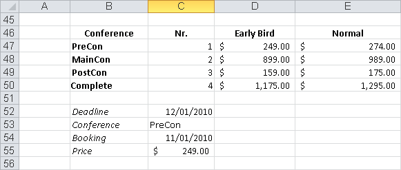
To calculate the price based on the elements booked and the reservation date, you use the following formula:
=INDEX((D47:D50,E47:E50),VLOOKUP(C53,B47:C50,2,FALSE),,IF(C54<C52,1,2))
You divide the price range into two parts (don’t forget to put the reference in parentheses), calculate the course element with VLOOKUP(), and use this number as the row index. You don’t need a column index, because each range includes only one column. The IF() function compares the booking date with the deadline to determine the range to be searched.
Working with Cells in Named Ranges. With INDEX(), you can address specific cells in a named range. This is especially useful for dynamic ranges. You can find more examples of this in the section for the OFFSET() function.
Assume that you want to add up the last cells in the lower-right corners of two ranges. The ranges are named NumberOne and NumberTwo, and their size is unknown. You can use the reference version
=INDEX((NumberOne,NumberTwo),ROWS(NumberOne),COLUMNS(NumberOne),1)+
   INDEX((NumberOne,NumberTwo),ROWS(NumberTwo),COLUMNS(NumberTwo),2)
as well as the array version
=INDEX(NumberOne,ROWS(NumberOne),COLUMNS(NumberOne))+
   INDEX(NumberTwo,ROWS(NumberTwo),COLUMNS(NumberTwo))