Syntax. BINOM.DIST(number_s;trials;probability_s;cumulative)

Definition. This function returns the probabilities of a binomial distributed random variable. Use the BINOM.DIST() function for problems with a fixed number of tests or trials when the results of a trial are only success or failure, when trials are independent, and when the probability of success is constant throughout all trials. For example, you can use the BINOM.DIST() function to calculate the probability that 50 of 100 people in a restaurant support a smoking ban.

Arguments

Background. In general, the probability can be defined as the likelihood that an event will occur when running a random trial where none of the given events is favored.

For example, how high is the probability that 30 packages will be damaged when producing 2,000 pills if it is assumed that 2 percent of the packages will be damaged?

Random trials for which a random variable can fall in one of two categories are usually called Bernoulli experiments, named for the Swiss mathematician Jakob Bernoulli (1654–1705).

The random variable (Bernoulli variable) x has the value x=1 with probability p (success) and the value X=0 with probability q=1-p (failure). The probability p is also called the success rate.

You often encounter events where the outcome can be divided into two categories. Therefore, a series of n Bernoulli experiments exists. The probability that the random variable x=1 occurs in k cases is calculated with the following Bernoulli formula:

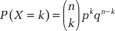
The distribution

of the random variable is called binomial distribution, with the binomial coefficient

—that’s n over k.

Binomial distribution is one of the most important probability distributions and is a special case of the multinomial distributions. Binomial distribution describes the results from Bernoulli processes, which in turn are defined as multiple Bernoulli experiments run under consistent conditions (for example, the toss of a coin).

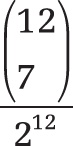
If you toss a coin, the probability of success and failure is the same. However, if you toss the coin 12 times, you get 2¹² possible results.

Example. The result of seven “heads” means that seven of the 12 results have “heads” as a single result. Choosing seven objects out of 12 is possible in many ways:

Therefore, the probability for seven heads results equals

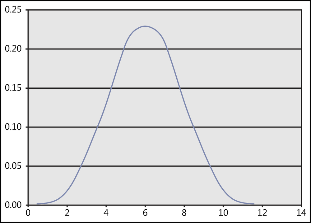
Excel provides the BINOM.DIST() function to calculate the probability of a binomial distributed random variable. Figure 12-15 shows an example of a binomial distribution.

Figure 12-15. Binomial distribution for p=0.5 and n=12.

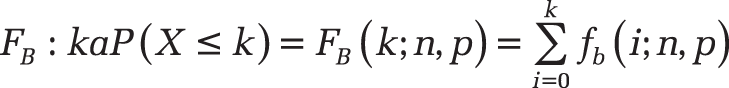
The density function of the binomial distribution is

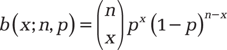
where

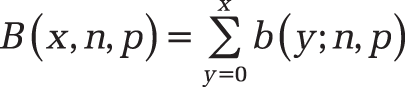
is COMBIN(n;x). The distribution function of the binomial distribution is

Examples

Vacation Directions. You are on vacation in a foreign city and ask a passerby for directions to a certain location. The question “Do you know the way?” can be answered only with yes or no. This means that there is a probability of 50 percent that the answer will be yes. Therefore, p is 0.5.

You want to know the probability that 66 of the 100 respondents (2/3) will answer yes. Figure 12-16 shows the calculation of the probability for the binomial distributed random variable 66.

Figure 12-16. Calculating the probability for a binomial distributed random variable.

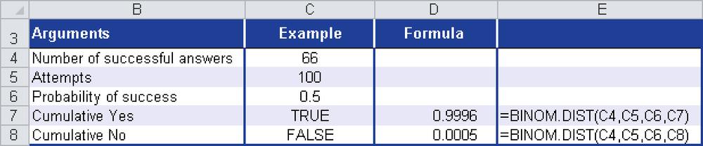
Here are the results:

In this way you can calculate many different probabilities.

Damaged Packages. Let’s use the example for the BINOM.DIST() function. The question in that example was: How high is the probability that 30 packages will be damaged when producing 2,000 pills if it is assumed that 2 percent of the packages will be damaged? Figure 12-17 shows the result.

Figure 12-17. BINOM.DIST() returns the probability for a binomial distributed random variable.

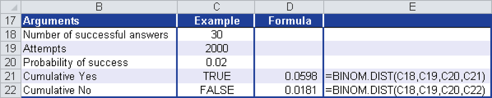
Here’s what you have discovered: