
Note
In Excel 2010, the FINV() function was replaced with the F.INV.RT() function, and the F.INV() function was added to increase the accuracy of the results.
To ensure the backward compatibility of F.INV.RT(), the FINV() function is still available.
Syntax. F.INV.RT(probability,degrees_freedom1,degrees_freedom2)
Definition. The F.INV.RT() function returns the inverse of the right F-distribution. If p = F.DIST.RT(x,...) then F.INV.RT(p,...) = x.
The F-distribution can be used in an f-test to compare the variances in two data sets. For example, you can analyze income distributions in the United States and Canada to determine whether the two countries have similar income diversity.
Arguments
probability (required). The probability associated with the F-distribution
degrees_freedom1 (required). The degrees of freedom in the numerator
degrees_freedom2 (required). The degrees of freedom in the denominator
Note
If one of the arguments isn’t a numeric value, the F.INV.RT() function returns the #VALUE! error.
If probability is less than 0 or greater than 1, the F.INV.RT() function returns the #NUM! error.
If degrees_freedom1 or degrees_freedom2 isn’t an integer, the decimal places are truncated. If degrees_freedom1 is less than 1 or degrees_freedom2 is greater than or equal to 1010, the function returns the #NUM! error. If degrees_freedom2 is less than 1 or degrees_ freedom2 is greater than or equal to 1010, the function returns the #NUM! error.
F.INV.RT() can be used to return critical values from the F-distribution. For example, the output of an ANOVA (analysis of variance) calculation often includes data for the F-statistic, F-probability, and critical F-value at the 0.05 significance level. To calculate the critical value of F, pass the significance level as the probability argument to F.INV.RT().
If probability has a value, F.INV.RT() looks for the value x so that F.INV.RT(x, degrees_ freedom1,degrees_freedom2) = probability. Therefore, the accuracy of F.INV.RT() depends on the accuracy of F.DIST.RT(). The function F.INV.RT() uses an iterative search technique. If the search has not converged after 100 iterations, the function returns the #N/A error.
Background. As already mentioned, the output of an ANOVA calculation often includes data for the F-statistic, F-probability, and critical F-value at the 0.05 significance level. This function performs a simple variance analysis to evaluate the hypothesis that the means of two or more samples are equal. The function can also test the significance of the differences in the arithmetic means of these groups to check if the variance between means is random.
The F.INV.RT() function calculates the critical value of a distribution. To calculate the critical value, pass the significance level as the probability argument to F.INV.RT().
The calculation of F.INV.RT() allows you to draw a conclusion regarding the null hypothesis. The arguments of the F.INV.RT() function are probability (for example, significance level a), degrees_freedom1, and degrees_freedom2.
Example. You work as an occupational therapist and want to find out to what extent employees identify with a company. You have selected 15 employees. Each employee answered 10 questions on other subject areas. For each question, the employees could choose between three answers.
You have already summarized the answers (see Figure 12-46).

The null hypothesis is that there is no difference between the three groups. The alternative hypothesis assumes the opposite. The significance level is 0.05 percent. Figure 12-47 shows the result of the univariate variance analysis.
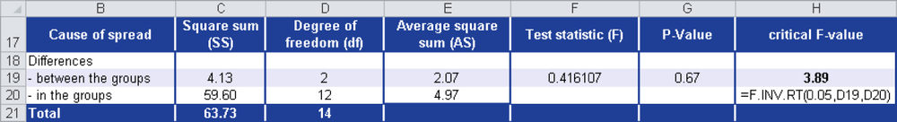
The result distinguishes the differences between the groups and the differences within groups, because not only are the three groups different but also the results of the employees within a group are different.
The differences between the groups correspond to the evaluated difference, and the differences within a group are random.
The number of degrees of freedom 1 (degrees of freedom within the groups) is calculated based on the size of the three groups minus 1 (5 – 1 + 5 – 1 + 5 – 1 = 12). The number of degrees of freedom 2 (degrees of freedom between the groups) is calculated based on the number of groups minus 1 (3 – 1 = 2).
The value for statistic F is 0.42 (cell F19). When you compare this value with the critical F-value calculated by F.INV.RT(), you can draw a conclusion regarding the null hypothesis. If the value of the calculated statistic F is greater than or equal to the critical F-value, the null hypothesis is rejected. In this example, the null hypothesis is accepted, because there is no significant difference between the three groups.