
Syntax. POISSON.DIST(x,mean,cumulative)
Definition. This function returns the probabilities of a Poisson distributed random variable. A common application of the Poisson distribution is the prediction of the number of events over a specific time period such as the number of calls a call center receives within an hour.
Arguments
x (required). The number of events.
mean (required). The expected numeric value.
cumulative (required). The logical value that represents the type of the function. If cumulative is TRUE, POISSON.DIST() returns the cumulative Poisson probability that the number of random events occurring will be between zero and x inclusive. If cumulative is FALSE, the function returns the probability that the number of events occurring will be exactly x.
Note
If x isn’t an integer, the decimal places are truncated. If x or mean isn’t a numeric expression, the POISSON.DIST() function returns the #VALUE! error. If x is less than 0, the function returns the #NUM! error. If mean is less than or equal to 0, the function returns the #NUM! error.
Background. The POISSON.DIST() function (named after Denis Poisson, 1781–1840) returns the probabilities of a Poisson-distributed random variable. The Poisson distribution predicts the frequency of independent similar events from a large number of elements.
An example is the number of customers arriving at a plaza or the number of incoming phone calls.
The Poisson distribution is especially useful for probability distributions with many results from a sample and a low probability for the event to occur. In this case, the Poisson distribution is similar to the binomial distribution. Unlike the binomial distribution, the Poisson distribution (in addition to x) requires only one parameter—the expected value or the mean argument.
For low probabilities, the binomial distribution approximates the Poisson distribution. This means that the distribution applies if the average number of events is the result of a large number of event possibilities and a low number of event probabilities. Radioactive decay is often used as example. In a very large number of atoms, only a very small amount of atoms decay within a time interval. The decay is random and independent from the already decayed atoms. This is an important requirement for the Poisson distribution.
The Poisson distribution assumes that the event occurs rarely within a certain time interval. However, the distribution depends only on the length of the interval and is independent of the position on the time axis. Therefore, you can use the Poisson distribution to calculate the error probability or one event per interval.
The POISSON.DIST() function calculates the following formulas:
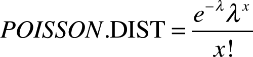
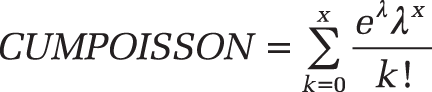
For these formulas, the POISSON.DIST() function replaces x with the number of events and mean with the expected number value. The cumulative argument indicates whether the mean is reached exactly (cumulative = FALSE) or at the most (cumulative = TRUE).
Example. You are a tire dealer and sell your own brand. You have analyzed the quality of your brand over a long time period. It has turned out that with your tires, an average of four incidents of tire damage per 100,000 miles occur (see Figure 12-114).
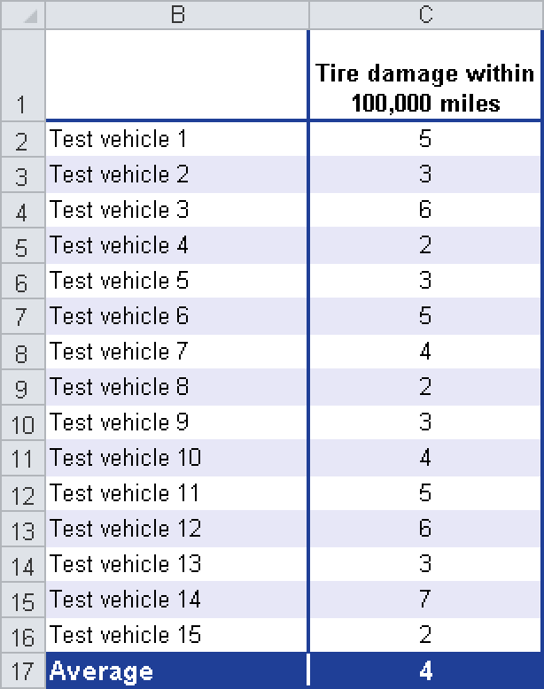
Compared with the interval of 100,000 miles, these four events are rare events. Therefore you use the Poisson distribution. You ask the following question: How high is the probability for only three tire-damage incidents per 100,000 miles to occur?
You enter the following values for the arguments required by the POISSON.DIST() function:
x = 3 (number of events you want to evaluate)
mean = 4 (number of expected events)
cumulative = FALSE (because you want to calculate the probability of x events to occur)
Figure 12-115 shows the result.
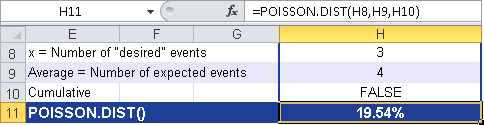
The POISSON() function returns a probability of 19.54 percent that three tire damage incidents per 100,000 miles will occur. To calculate the probability of 0 to x tire damage incidents per 100,000 miles, specify the logical value TRUE for the cumulative argument (see Figure 12-116).
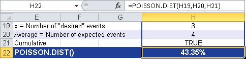
The POISSON.DIST() function returns a probability of 43.35 percent for 0 to 3 tire damage incidents per 100,000 miles to occur.