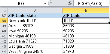
Assume that you have an address list in which one column contains a location consisting of the state and a five-digit ZIP Code. You do not need the state but want to pick up just the five-digit ZIP Code. Therefore, you need to query for the last five characters of the complete address.

Assuming that cell A38 contains the address, the formula reads:

=RIGHT(A38,5)

In this case, the RIGHT() text function returns the five characters at the right end of the string (see Figure 2-9).

Figure 2-9. The five-digit ZIP Code is extracted with the RIGHT() table function.

Assume that a list of names contains both the first and last name. Separating the first names from the last names is more difficult than extracting the five-digit ZIP Code, because the names are not of standard length.

Assuming that cell A21 contains the first and last name separated by a space, enter the following formula in B21 to extract the first name (Figure 2-10):

=LEFT(A21,FIND(" ",A21)-1)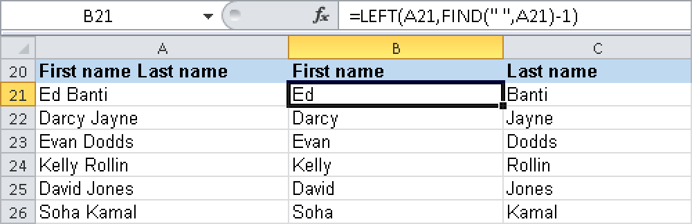

Figure 2-10. The first name is extracted by specifying the separator.

Because first names are different in length, you have to use the FIND() function to find the first space. This function returns the position of the space in the text as a number. This number is decreased by 1 and used in the LEFT() function as an argument for the number of characters to return the first name.

To extract the last name, enter the following formula in cell C21:

=RIGHT(A21,LEN(A21)-FIND(" ",A21))

The RIGHT() function extracts the last name. To calculate the number of characters to extract from the right, you use the length of the entire name and subtract from this the number of characters in the string up to the first space, using the FIND() function again to find the position of the space. But this is not sufficient. It would be a coincidence if the space was at the same position as the number of characters read from the right.

Therefore, you use the LEN() function. This function identifies the total number of characters in the text. If you subtract the position number of the space from the total number of characters, as in LEN(A21)-FIND(“““,A21), you get the length of the last name.

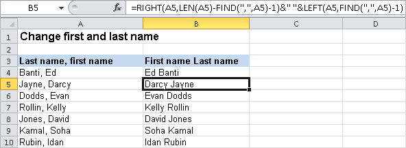
If in one column the last name is placed in front of the first name, you may want to reverse the order. Assume that cell A5 contains the name Jayne, Darcy. As long as the order of the last names and first names is the same and the separator is a comma and a space, you can use the following formula to switch the names:

=RIGHT(A5,LEN(A5)-FIND(",",A5)-1)&"  "& LEFT(A5,FIND(",",A5)-1)

The result is Darcy Jayne (see Figure 2-11).

The first name is extracted by using the function

=RIGHT(A5,LEN(A5)-FIND(",",A5)-1

Note that the FIND function finds the position of the comma, and a further character must be subtracted to allow for the space after the comma. The last name at the beginning of the text string uses the function

=LEFT(A5,FIND(",",A5)-1)

Then the two names are concatenated together, with a space as a separator, using

& " " &

Figure 2-11. Nested but effective—switching names by using a formula.

The IBAN (International Bank Account Number) is required for international money transactions. Because this number consists of parts with a fixed length, you can pick out individual components of the IBAN. The IBAN can be up to 34 characters long. A German IBAN consists of 22 characters in the following order (see Figure 2-12):

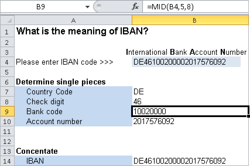
To separate out the parts of the IBAN in cell B4, use the following formula:

You have already used the LEFT() and RIGHT() functions in the previous examples. To extract strings from the middle of a text string, use the MID(text,start_num,char_num) function.

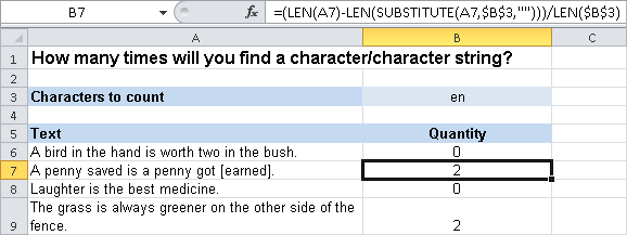
For journalistic tasks and text analysis, it might be necessary to determine how often a certain character or string appears in a block of text. With the following trick, you can do this in Excel: If cell B3 contains the string and cell A7 contains the text to be analyzed, use the following formula:

=(LEN(A7)-LEN(SUBSTITUTE(A7,$B$3,"")))/LEN($B$3)

The LEN(A7) function calculates the number of characters in cell A7. The SUBSTITUTE() function in the second part of the formula replaces any occurrence of the characters in the test string with nothing (“”) and calculates the new length. If you subtract this length from the original length of the string and divide by the length of the test string, you will calculate the number of occurrences (see Figure 2-13).

Figure 2-13. The trick for counting the frequency of characters.

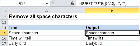
In some cases, you may want to remove blank characters from a text string. To do this, you can use the SUBSTITUTE() function (see Figure 2-14). If you want to remove all spaces from the text in cell A15, for example, you can use the following formula:

=SUBSTITUTE(A15," ","")

Figure 2-14. The SUBSTITUTE() function replaces strings.

Here is the function with its syntax:

SUBSTITUTE(text,old_text,new_text,[instance_num])

This function replaces the old text with the new text in a string. In this example, the space (“ “) is replaced with an empty string (“”). New York becomes NewYork. You can also use the SUBSTITUTE() function to replace certain characters in a text string.

When you are importing data, sometimes the minus sign for negative numbers appears after the value. Because Excel doesn’t accept this expression as a number, it cannot be used in calculations. In fact, the position of the minus sign leads to the number being interpreted as a text value.

To convert the value in cell A4 into a number, use the following formula (see Figure 2-15):

=IF(RIGHT(A,1)="-",LEFT(A4,LEN(A4)-1)*(-1),A4)

Figure 2-15. Converting a number by changing the placement of the negative sign.

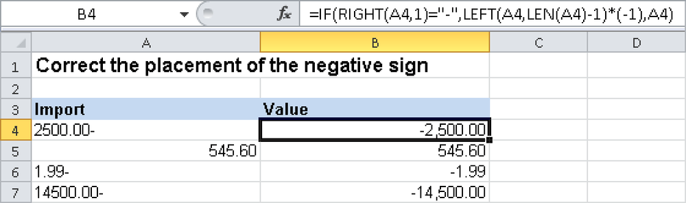
The IF() function is used to verify the content of parts of a cell. The RIGHT() function checks whether a minus sign is present. The LEFT() function separates the number part and converts it into the negative value of the number by multiplying it by –1.

The following formula displays the name of the current file. Enter the following formula in cell A21:

=CELL("filename")

This function returns the file name of the current worksheet; the full file path and sheet name are displayed. If the current worksheet has not yet been saved, the function returns an empty string.

Within the string, the file name is enclosed in brackets, which can be useful in extracting the name from the string. The following formula extracts the file name from the result:

=MID(A21,FIND("[",A21,1)+1,FIND("]",A21,1)-FIND("[",A21,1)-1)

The MID() function calculates the number of characters from the start position. The FIND(“[“,A21,1)+1 expression determines the start position after the left bracket. The FIND(“]”,A21,1)-FIND(“[“,A21,1)-1 expression calculates the number of characters between the left and the right brackets.

You can also use this function to display the name of the worksheet. To do this, use the following formula:

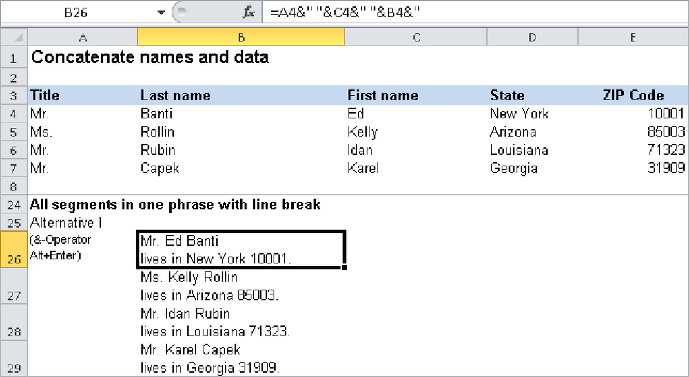
=MID(A21,FIND("]",A21,1)+1,LEN(A21))

Figure 2-16 shows a typical address list. To concatenate the data in the list, use the following formula:

=A4 & " " & C4 & " " & B4 & " lives in " & D4 & " " & E4 & "."

Figure 2-16. The & concatenation operator combines text and values in more complex expressions.

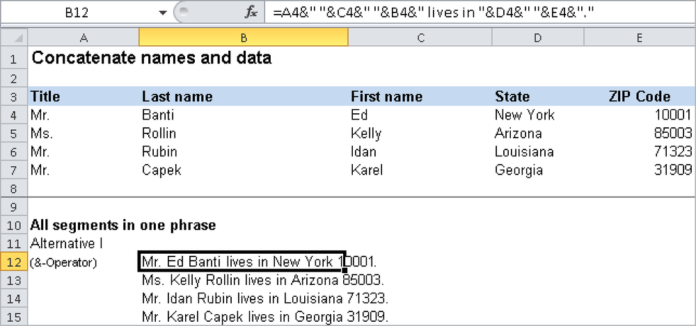
You can concatenate text and references with the & concatenation operator. You can also use the CONCATENATE() text function, which returns the same result.

=CONCATENATE(A4," ",C4," ",B4," lives in ",D4," ",E4,".")

For some text concatenations, you might want to insert a line break in a place other than at the right margin, such as after a certain number of characters or after a certain word. You can press Alt+Enter to insert the break at any position. As soon as you press the Enter key, the line break is visible in the cell.

You can also link two strings with a newline character (see Figure 2-17). The newline character has a character code of 10 and can be added with the CHAR() function:

=CONCATENATE(A4,"  ",C4,"  ",B4,CHAR(10),"lives in  ",D4,"  ";E4;".")

Figure 2-17. Text concatenations can contain line breaks and other special characters.

You probably use Excel charts to present numbers. However, you can use in-cell graphics instead of charts to display data. To do this, you can use the REPT() function, as shown in Figure 2-18.

Figure 2-18. Creating graphics with the REPT() function.

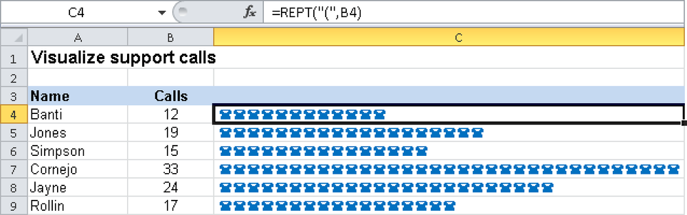
In this example, the calls answered by the support personnel are captured in a list. The formula

=REPT("(",B4)

converts the number 12 in B4 into twelve phone icons. You will need to select the Wingdings font for the formula cell to display the opening parenthesis as a phone icon.