

The table structure of Excel worksheets allows the user to systematically search worksheets for information.
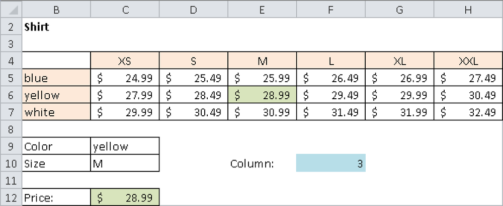
Assume that you have tabulated price information for an item (in this example, shirts in different colors and sizes). After selecting a color and size, you want to look up the price and use this price in further calculations (see Figure 2-21). To do this, you use a typical cross tabulation.
Excel offers a range of lookup functions that can be used for this kind of task. There are three main functions: LOOKUP(), VLOOKUP(), and HLOOKUP(), as well as the MATCH() and INDEX() functions, which provide similar facilities. All of these functions find information in a rectangular area according to some criteria and return the information or the position of the information from the table. The following examples demonstrate how some of these functions can be used.
See Also
You will find detailed descriptions of the other functions in Chapter 10.
The VLOOKUP() function takes a value and tries to match it to values in the first column of a table. When a match is found, the function will return any of the information associated with the item matched in the table. There are two ways that it can perform the search:
Look for an exact match of the item in the first column of the table.
Look for a value, either the exact value or the value nearest to but lower than the value being searched for. In this case, the lookup table must be sorted on the first column.
The MATCH() function searches an array of values and returns the position of the first match in that array, either the column or the row. Matches can be exact, or the lowest or highest value.
Figure 2-21 shows the prices for shirts in different colors over a range of sizes. You are searching for information not only in a certain row but also in a certain column. Just proceed one step at a time. First, find the column containing the required size. The third column contains size M. If you want Excel to recognize this, press F10 to enter 3 in an auxiliary cell. The formula =MATCH(C10,C4:H4,1) finds the value in cell C10 (size M) in the heading of cells C4 through H4 and returns the column number. Chapter 10 explains these functions in detail.
The second step is achieved by using the VLOOKUP() function. Enter the following formula in cell C12:
=VLOOKUP(C9,B5:H7,F10+1,FALSE)
This formula searches for the content of cell C9 (yellow) in the first column of cells B5 through H7. If a value is found, the formula returns the value in the fourth column. The job is done!
There are several things that you can do to make this more elegant. Instead of using two formulas, you can embed the MATCH() function into the VLOOKUP() function to get the result from a single formula. Conditional formatting would provide a nice feature to emphasize the selected cell.
Another popular function in this category is the OFFSET() function. This function focuses on a specific range and allows you to dynamically adjust this by defining row and column offsets.
Take a look at the following example (see Figure 2-22), in which daytime temperatures are tabulated over a five-day period. Assume that you want to display the daytime temperatures for a selected day.
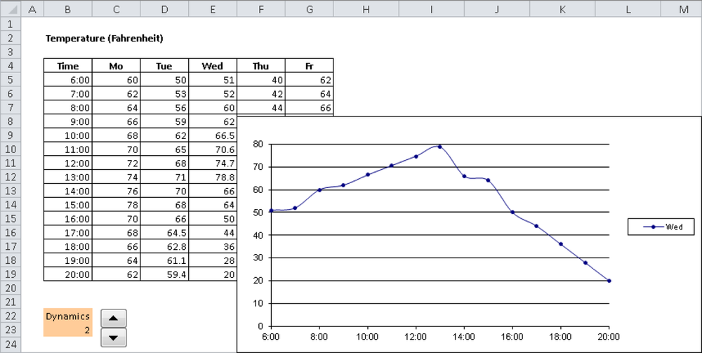
The solution is to dynamically link the column used by the temperature chart to an input value on the worksheet. Start by creating a line graph to display the temperatures throughout the day for Monday.
There are some tricks you can use. First, you can name not only ranges but also formulas. In Excel 2007 and Excel 2010, on the Formulas tab, select Defined Names/Define Names, and in previous versions select Insert/Names/Define to name formulas. Use these to define dynamic ranges for the legend and the data series for the chart. Define the name chartDay as:
=OFFSET(charts!$C$4,0,charts!$B$23)
The reference in cell C4 on the Charts worksheet is moved zero rows down and the number of columns to the right as indicated in cell B23 (see Figure 2-22).
Do the same for the chart data. Use the name chartData and link it with the formula
=OFFSET(charts!$C$5:$C$19,0,charts!$B$23)
This formula applies to the entire column instead of to only one row. The reference is moved in the same way. After the chart is created, click the drawn line. Something similar to the following is displayed in the input box:
=SERIES(charts!$C$4,charts!$B$5:$B$19,charts!$C$5:$C$19,1)
Change this entry by replacing the absolute cell references with your dynamic references:
=SERIES(Lookup.xlsx!chartDay,charts!$B$5:$B$19,Lookup.xlsx!chartData,1)
You have to use the name of the workbook, and the names have to be separated by an exclamation mark. For a perfect solution, you should also add a spinner control to select the value in cell B23.