Similar to the logical functions, the information functions serve to supplement and support other functions and formulas.

At the center of the information functions are the so-called IS functions (see Table 2-2), which provide information about expression types or the cell content. This information can be viewed or, more usefully, used for other calculations. The names of these functions are self-explanatory, and the returned values are always logical values. The logical value confirms whether the value of the cell specified in the argument is of the required type. Usually the argument for the functions is a cell reference, but sometimes—for example, for the ISREF() function—a specific value is provided for testing.

When you work with named ranges and use these ranges as references, you get a #REF! error if you accidentally delete the name. For example, assume that cells B2 through D5 have the name Sales, and that cell F7 contains

=SUM(sales)

This works as long as the name Sales exists. However, the formula

=IF(ISREF(sales),SUM(sales),"Name Sales was removed.")

is somewhat safer. The ISREF(sales) function returns FALSE if the name Sales is removed. Instead of calculating the sum for the unknown range and generating an error, Excel displays a message stating the cause of the error. If the range name exists, the total is calculated.

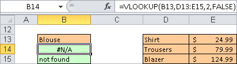
Errors can often occur when you are using the VLOOKUP() function, particularly when you are searching for an item that is not in the list. In Figure 2-23, the formula

=VLOOKUP(B13,D13:E15,2,FALSE)

generates an #N/A error (N/A=not available) indicating that the Blouse item is not in the list. The formula

=IF(ISERROR(VLOOKUP(B13;D13:E15;2;FALSE)),"not found", VLOOKUP(B13;D13:E15;2;FALSE))

is longer, but it first verifies whether VLOOKUP() was successful. If it was not, the message “not found” appears; if the function was successful, the price is displayed.

Figure 2-23. Searching for information in lists.

Often simple calculations can lead to errors; consider, for example, the use of a function such as 1/x (x cannot be zero) or LOG(x) (x has to be positive). If you want to create a chart from a series of numbers, you can manipulate the data to ensure that incorrect values “disappear” from the source range of the chart.

Figure 2-24. This presentation of 1/x is incorrect because the error values are shown as zero.

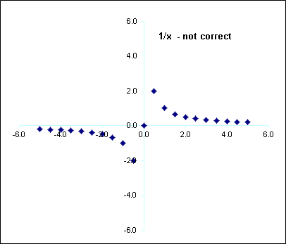
To avoid the incorrect presentation in Figure 2-24, enter

=IF(ISERROR(1/B13),NA(),1/B13)

This way you intercept the #DIV/0! error and replace it with the NA() function that indicates that the value doesn’t exist. Do the same for other error values.