
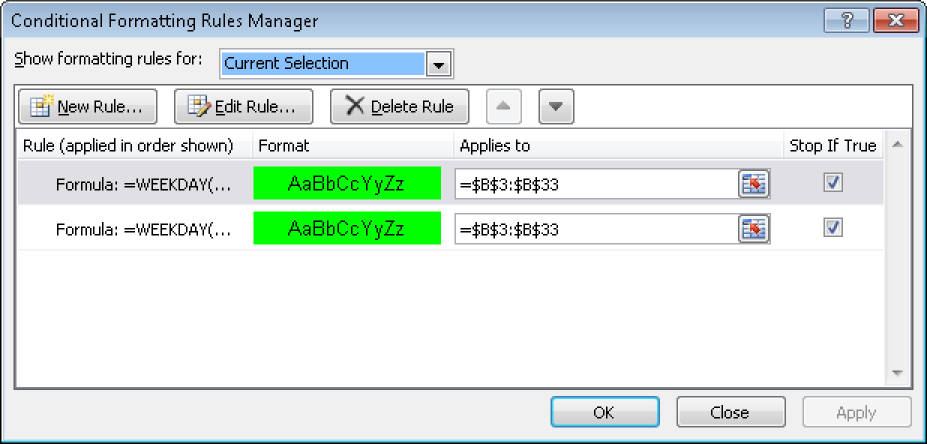
Excel 2003 offered a range of conditional formatting options with up to three rules. This feature has been greatly improved in Excel 2007 and Excel 2010, and now offers an unlimited number of rules. Also, in addition to standard formatting, you now have a range of color scales, data bars, and icons to choose from. There is also a Rules Manager, offering a much improved way to define and manage the rules (see Figure 5-5).
In addition to simple data range selections, conditional formatting can also be applied to formulas.
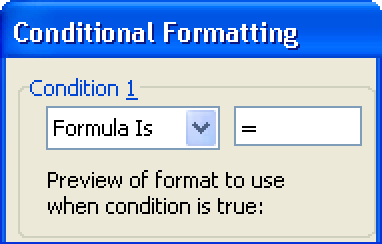
In Excel 2003, select Formula Is in the left side of the Conditional Formatting dialog box (see Figure 5-6) and enter the formula in the field to the right. The formulas must return the value TRUE or FALSE. If the formula returns TRUE, the formatting is applied according to your settings.
In Excel 2007 and Excel 2010, on the Home tab, click the Conditional Formatting button and select New Rule. Then select the Use A Formula To Determine Which Cells To Format rule type.

With the ability to use a formula to set conditional formatting, the range of functions available in Excel, and the unlimited number of rules in Excel 2007 and Excel 2010, the possibilities are endless. The following examples explore just a few of the capabilities.
Note
The Chapter05_CF.xlsx workbook in Excel 2007 and Excel 2010 file format, and the additional New in Excel 2007 and Excel 2010 sheet, show the new possibilities based on the temperature example in the section later in this chapter, Emphasizing the Top Three Elements.
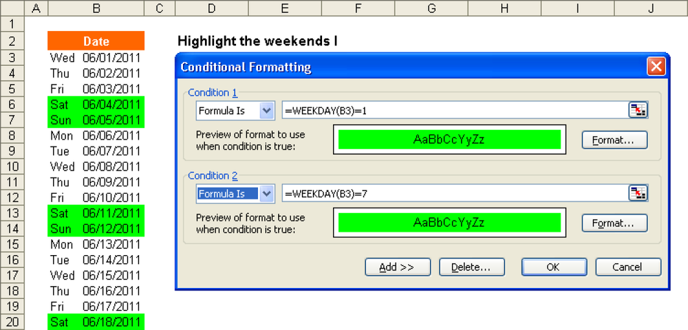
Assume that you want to highlight Saturdays and Sundays as weekends in a column containing dates. Use the WEEKDAY() function in Excel to return the weekday for a date value (see Chapter 7, for more information) where a value of 1 corresponds to Sunday, and 7 corresponds to Saturday. This can be used to set a light green background for weekends by using the conditional formatting options.
Assume that the range B3:B33 contains the dates for one month. Select this date range, and then follow these steps:
For Excel 2007 and Excel 2010:
Select the date list and then select Conditional Formatting, New Rule, and Use A Formula To Determine Which Cells To Format.
Enter the following formula in the input field:
=WEEKDAY(B3)=1Click the Format button and, in the Format dialog box, select the Fill tab. Select light green as the color.
Confirm the format and the condition by clicking OK.
Repeat these steps to add another rule, but this time use the formula
=WEEKDAY(B3)=7to highlight Saturdays.
Select the date list and, on the Format menu, select Conditional Formatting.
In Condition 1, change the option Cell Value Is to Formula Is and enter the following formula in the input field:
=WEEKDAY(B3)=1Click the Format button and, on the template, select light green as the color.
Click Add to add a further condition, and repeat the previous steps, entering
=WEEKDAY(B3)=7in the input field of Condition 2.
Using a combination of conditional formats and Excel functions is a useful way to visually highlight information. Figure 5-7 shows the completed dialog box and the result for the date list.
Another possibility is to combine the two conditions with an OR function if the same formatting is to be used in both instances. With the logical function OR() (see Chapter 9), you need only one condition:
=OR(WEEKDAY(B3)=1,WEEKDAY(B3)=7)
This is particularly useful in Excel 2003, in which the number of conditions is limited.
Alternatively, the TEXT() function could be used to determine the day rather than WEEKDAY():
=OR(TEXT(B3,"ddd")="Sun",TEXT(B3,"ddd")="Sat")
In this formula, the “ddd” formatting command returns the first three letters of the weekday.
Color-highlighting weekends in calendar overviews is useful, but what about other days, such as national and cultural holidays? It also might be useful to automatically highlight days such as payment dates, deliveries, maintenance, and monthly or quarterly reports.
These dates can be added to a list to be considered for highlighting. In our example, besides processing weekends, two more requirements have to be met: holidays and other free days. This means that four conditions have to be checked:
Saturdays
Sundays
Holidays
Other free days
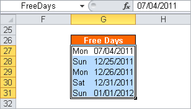
Start by setting up the Free Days list. Enter the information into the spreadsheet and name the list.
Select the range G27:G31 and click in the Name Box.
Enter the name FreeDays.
Press the Enter key.
Figure 5-8 on the next page shows the result. The highlighted range now has the name FreeDays.
To check whether a date is included in the Holidays range, you need to use the MATCH() function. This function has the following syntax:
=MATCH(Lookup_value, Lookup_array, Match_type)
The lookup_value is each cell of the date list. The lookup_array is the FreeDays range. Match_type specifies how Excel is to match the matrix values with the lookup_value. This example uses the type 0 for an exact match. Data in the lookup_array does not need to be sorted.
The MATCH() function returns a number for the position of the value found in the lookup_array. If the date is not contained on the FreeDays list, the error value #N/A is returned.
Finally, the ISNUMBER() function is used to determine whether a match has been found. If the MATCH function returns a numeric value, the date is included on the FreeDays list.
=ISNUMBER(MATCH(B3,FreeDays,0))
Add this condition to the conditional formatting already set to highlight weekend days. Assign the free days a red background color and a bold white font color in contrast
Select the date range and invoke conditional formatting.
Don’t change the rules currently set for weekends. Click New Rule (or Add, in Excel 2003).
Select Formula Is again, and enter the formula
=ISNUMBER(MATCH(B3,FreeDays,0))Click the Format button, and set the background and font colors.
Click OK.
The result is shown in Figure 5-9.
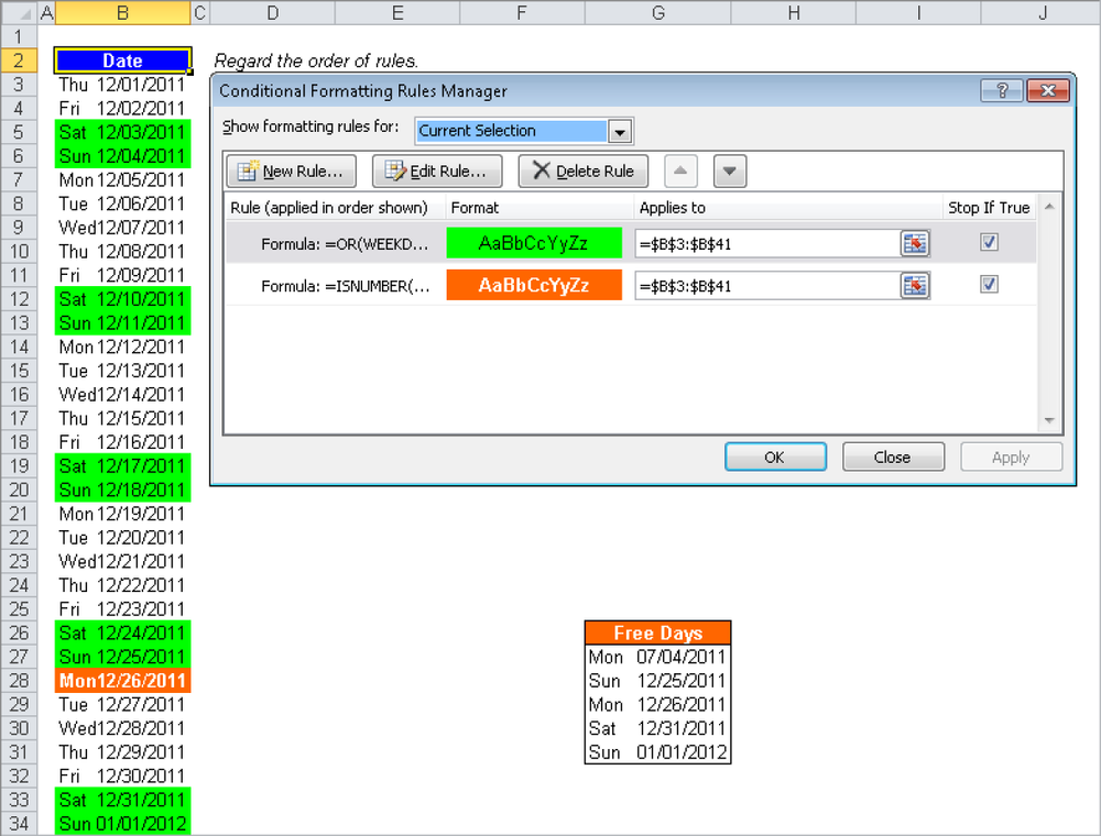
Note that the order of the conditional formatting conditions is important. The formatting will be applied sequentially, so if the Free Days condition is checked first, the holiday format will be applied rather than the weekend format for a holiday that falls on a weekend. Reverse the conditions to give preference to the weekend formatting. In Excel 2007 and Excel 2010, with the Conditional Formatting Rules Manager, you can move rules up and down in order. In Excel 2003, each condition will need to be reset.
The example of the calendar overviews demonstrates some of the facilities available for highlighting information.
Note
When you are editing the formula in the condition formula box, using the arrow keys may change the cell referencing instead of moving the mouse pointer along the edit box. To avoid this, activate the input field for the formula and press the F2 key to switch from Point mode to Edit mode. Now the arrow keys should work as expected.
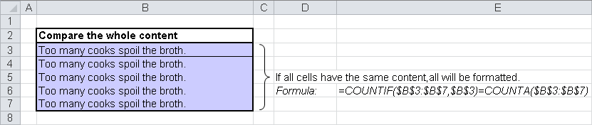
Sometimes it may be useful to highlight cells with identical content. Several functions are available to compare the content of cells, and conditional formatting can be used to highlight the results.
To format the cells in the range B3:B7 as light blue if all of the cells contain the same content (see Figure 5-10), perform the following steps:
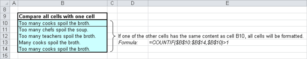
Let’s take a look at a different scenario: All cells in the range B10:B14 have to be formatted if the range B11:B14 includes a cell that matches cell B10. Perform the following steps:
All cells are formatted if the range B11:B14 contains a cell with the same content as cell B10 (see Figure 5-11).
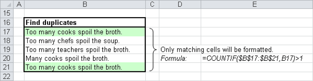
The following example also compares the cells in a range. It formats those cells in the selected range that have identical contents. Perform the following steps:
Cells are only formatted if they match the content in cell B17. The COUNTIF function counts the number of matches and if it is greater than 1, formatting is applied (see Figure 5-12).
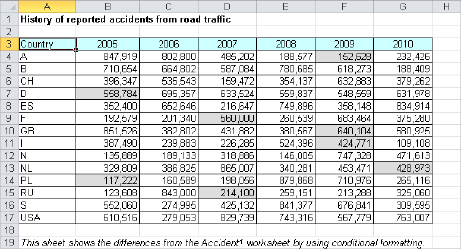
Sometimes you might have two versions of a table, and you want to compare them to see if there are any differences. Conditional formatting can help.
Assume that you have two versions of a worksheet containing accident statistics—Accident1 and Accident2. On the Accident2 worksheet, you want to highlight the cells that have different content from the matching cell or cells on Accident1.
This task should be simple, because you need to compare only the cell content. But there is a problem you need to consider. Try these steps:
You get an error message. Conditional formatting cannot handle external references to other worksheets or workbooks. The solution is to use a table function to calculate these references.
Note
Select a range big enough for comparison with conditional formatting to also highlight new or deleted records.
To use an external sheet reference for conditional formatting, do the following:
Select the Accident2 worksheet and select the data range.
Select the Conditional Formatting command and then Formula.
Enter the following formula as the condition:
=B4<>INDIRECT(ADDRESS(ROW(B4),COLUMN(B4),TRUE,TRUE,"Accident1"))Click the Format button and select the format you want.
Confirm the format by clicking OK.
Now the cells in which Accident2 differs from Accident1 are visible (see Figure 5-13). The functionality of the INDIRECT(), CELL(), and COLUMN() functions is explained in Chapter 11.
Note that the reference to the worksheet is entered as a string, which means that the formula is not automatically updated if the name of the worksheet changes. In this case, remember to modify the formula for conditional formatting.
This solution also works with tables in different workbooks, but both workbooks must be open. You can use the following formula to apply conditional formatting to reference an external workbook:
=B4<>INDIRECT(ADDRESS(ROW(B4),COLUMN(B4),TRUE,TRUE,"[Accident.xlsx]Accident 1"))
Note that the workbook extension in Excel 2003 is .xls.
If you print a list, it might be better to highlight every other row with a color rather than use borders (see Figure 5-14). But for large lists, it would be very tedious to format every other line manually, and a single sorting process would undo your work. Conditional formatting can help:
Select the list range without the titles.
Select Format/Conditional Formatting and then Formula Is (Excel 2003), or click the Conditional Formatting button on the Home tab, select New Rule, and then select Use Formula (Excel 2007 and Excel 2010).
For Condition 1 (Excel 2003) or Rules Description (Excel 2007 and Excel 2010), enter the formula
=MOD(ROW(),2)=1to highlight the rows with uneven numbers.
Click the Format button and select the format you want.
Confirm the format by clicking OK.
The functionality of the MOD() function is described in Chapter 16.
Even if the list is dynamic, the current formatting will always be applied to the same range. The formatting can be extended dynamically by combining two tests with the AND() function, as follows:
=AND(MOD(ROW(),2)=1,$A2<>"")
With this formula, conditional formatting also tests the first column of the list. If this column contains a value and the line number meets the condition, a reference line is displayed. To use this formula, select a larger range before you enter the condition. The formatting takes place only if this range is filled with data.
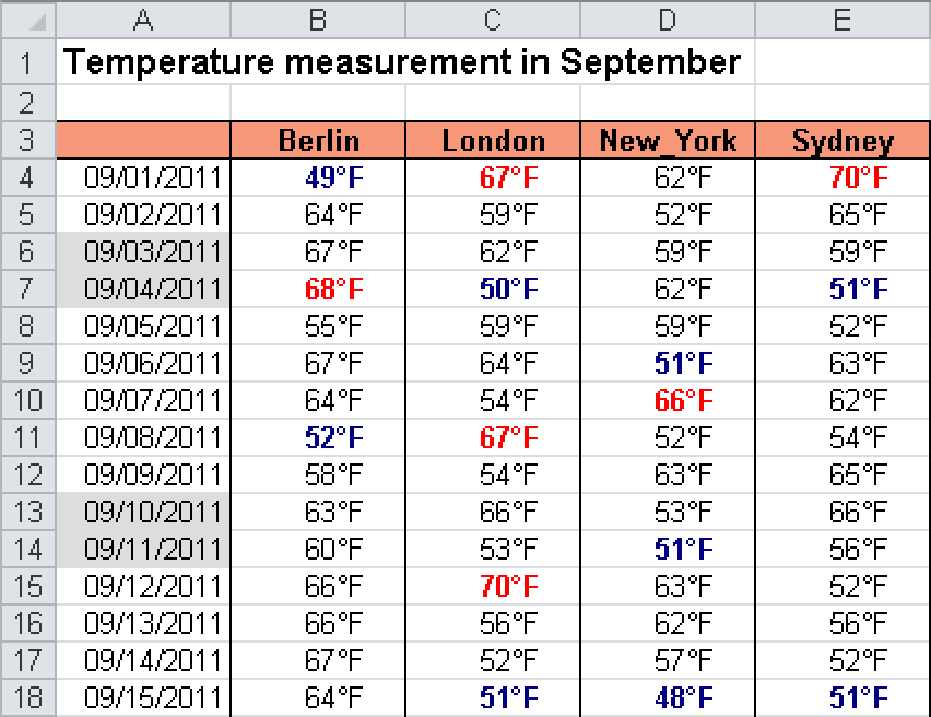
Emphasizing the top elements should not be a problem with conditional formatting. Assume that you measured the temperatures of different places for a month. You now want to emphasize the three warmest and the three coldest temperatures (see Figure 5-15).
To perform this task, do the following:
Select the columns containing the temperatures, including titles (in this example, the range B3:E33). Press Ctrl+Shift+F3 to open the Create Names dialog box.
Select the Top Row check box to create the names from the top row, and click OK to confirm.
The data columns now have range names (the strings in the titles). These are required for the formulas for conditional formatting.
Select the range with the temperatures (in this example, the range B4:E33) and select Conditional Formatting. In the Conditional Formatting dialog box, select Formula as the first condition and enter the following formula:
=OR(B4=MAX(INDIRECT(B$3)),B4=LARGE(INDIRECT(B$3),2),B4=LARGE(INDIRECT(B$3),3))Click the Format button and select a format on the Font tab (for example, bold and red). Click OK to confirm.
In Excel 2003, click the Add button, and in Excel 2007 and Excel 2010, click New Rule. Enter the following formula for the second condition or rule:
=OR(B4=MIN(INDIRECT(B$3)),B4=SMALL(INDIRECT(B$3),2), B4=SMALL(INDIRECT(B$3),3))Click the Format button and choose a format on the Font tab (for example, bold and dark blue). Click OK to confirm.
The INDIRECT() function creates the range names from the titles, which allows you to create conditional formats for all of the columns in one step. Chapter 12, describes the static MIN(), MAX(), SMALL(), and LARGE() functions in more detail.
Importing data from a text file can cause problems if the information contains blank characters, particularly if the cell content ends with a space, because this is not immediately obvious. Although you can search for spaces with the Find And Replace dialog box, it might not be possible to replace all spaces, because those in the center of a text string may be perfectly valid. The TRIM() function can be used to remove leading and trailing blanks, but a case-by-case review may be more useful. Conditional formatting can be used to highlight cells that contain blanks.
You can use conditional formatting for this purpose by applying the formulas shown in these examples:
=LEFT(C5,1)=CHAR(32). Identifies a leading space. C5 is the upper-left corner of the selected area.
=RIGHT(D5,1)=CHAR(32). Identifies a space at the end. D5 is the upper-left corner of the selected area.
=OR(LEFT(E5,1)=CHAR(32),RIGHT(E5,1)=CHAR(32)). Identifies a space either at the beginning or the end. E5 is the upper-left corner of the selected area.
=FIND(CHAR(32),F5)>0. Identifies any space. F5 is the upper-left corner of the selected area.
Often you might need to choose a value from a table at the intersection of a certain row and a certain column. In this example, we want to make sure that the installment amount and the number of partial payments can quickly be found (see Figure 5-16). On a piece of paper, you can use a ruler and pencil; on the screen, conditional formatting can help.
The PMT() table function calculates the installment amount in cell C9 with the following formula:
=PMT($C$5/12,C$8,-$B9)
The combination of absolute (interest) and relative references (payment periods and cash value) allows you to copy the formula for the range C9:J28. Chapter 15, describes the math functions for finances, especially PMT(), in more detail.
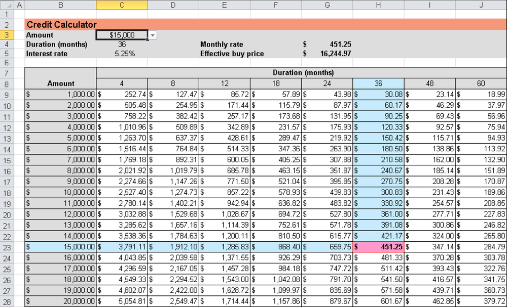
Using data validation, you can easily handle the input of the amount in cell C3 and the input of the duration in cell C4. For the input of the amount, use the named range Amount (this name stands for the range B9:B28), and for the input of the duration, use the named range Months (this name stands for the range C8:J8). The section titled Functions for Validation contains more examples of data validation.
To highlight the amount in column B:
Displaying the leader line is a bit more difficult. Several conditions have to be checked, because all of the cells in the row and all of the cells in the column should be formatted. You configure these conditions with the OR() function. Both conditions have restrictions, because each time, the formatting should only be applied up to a certain column or row. In this case, two conditions are valid and linked with the AND() function.
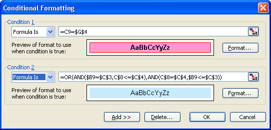
To highlight the result cell and insert leader lines into the data range, do the following:
Select the date range C9:J28 and select Conditional Formatting.
Select Formula and enter the formula
=C9=$G$4Select the format for the result cell, and click the Add button (or, in Excel 2007 and Excel 2010, the New Rule button).
Select Formula and enter the formula
=OR(AND($B9=$C$3,C$8<=$C$4),AND(C$8=$C$4,$B9<=$C$3))Select the format for the selected area, and confirm the format by clicking OK.
The order of the conditions is important. If the cell also corresponds to the result in the header, it should be highlighted as the result cell. Because this cell also meets condition 2, the formatting would never be displayed if the condition was the second condition.
Figure 5-17 shows the formulas for the conditions in the Conditional Formatting dialog box in Excel 2003.
Often large lists need to be sorted and separated. For example, a list containing information about several companies should be separated so that you can recognize associated groups quickly (see Figure 5-18). It is easy to do this manually, but can you do this dynamically, too?
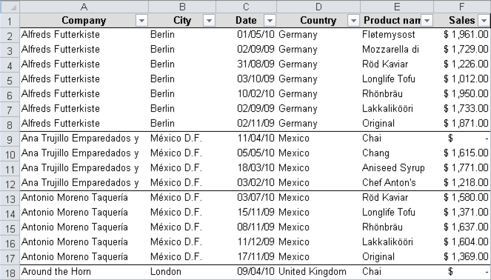
With conditional formatting, this task can be done dynamically:
Select the date range (the cells A2:F86 in this example).
Sort the data by company with the Data/Sort command.
Open the Conditional Formatting dialog box (New Rule).
In the dialog box, select Formula and enter the formula
=$A2<>$A3in the formula field.
Click the Format button and select the bottom border on the Border tab.
Close the dialog boxes by clicking OK.
This formula checks whether the value in the line that follows is the same as the value in the current line. If it is different, a separator line is inserted between the groups.
Suppose you have a list to which you have applied subtotals. Conditional formatting can be used to highlight the total lines (see Figure 5-19).
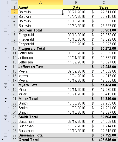
Perform the following steps to configure this format:
Use the Data/Sort command to sort the data by agent.
Select Data/Subtotal, and group the data by the Agent column.
Calculate the sum from Sales and click OK.
Select the data in the range A2:C30 and then select Conditional Formatting.
Enter the following formula:
=ISNUMBER(FIND("Total",$A2))Note the mixed reference for cell $A2!
In Excel 2007 and Excel 2010, the Conditional Formatting Rules Manager allows you to handle and manage conditional formats in an intuitive and a comfortable way. This section provides some hints for using conditional formats in Excel 2003 and previous versions.
To change a conditional format, select the cells you want to modify. Then open the Conditional Formatting dialog box and modify the setting for the individual conditions. Confirm the format by clicking OK.
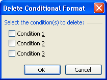
If you want to delete one or more conditions, select the corresponding cells and open the Conditional Formatting dialog box. Click the Delete button to open the dialog box shown in Figure 5-20. This dialog box contains three check boxes that you can select to indicate the condition you want to delete. Click the OK button to delete the conditions according to your settings.
Sometimes you might not know exactly which cells or cell ranges on a worksheet or in a workbook have conditional formats configured for them. In this case, Excel can help you with a little-known option.
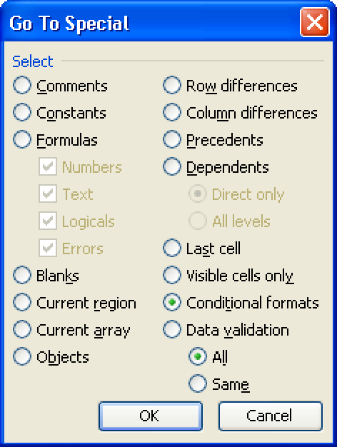
Press the F5 key to open the Go To dialog box (or select the Edit/Go To menu item, or press Ctrl+G).
Click the Special button.
Select Conditional Formats and, under Data Validation, select All (see Figure 5-21).
Start the operation by clicking OK.
With this approach, you can quickly delete or change the previously selected formats for all detected cells with conditional formats.
If you don’t want to find all of the cells with conditional formats but only those cells with exactly the same conditional formats, select Same under Data Validation.
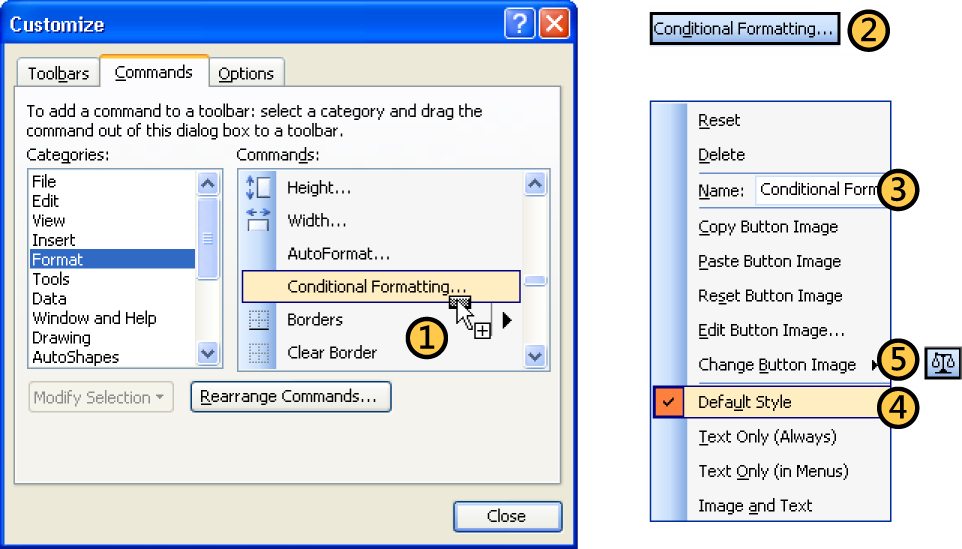
You access the Conditional Format command in Excel 2003 from the menu options. To add this command as an icon to your toolbars, follow these steps. Steps 1–5 correspond to the number labels in Figure 5-22.
On the Tools menu, choose Customize. Click the Commands tab and select the Format category. On the right side of the list, you should see the Conditional Formatting command without an icon.
Drag the Conditional Formatting option onto one of the existing toolbars.
Right-click the new button to open the shortcut menu. Give the new button a new label, if required.
Click the Default Style menu option.
Press the Enter key to confirm the changes.
Click Close in the Customize dialog box.
Now you can click the new icon to quickly open the dialog box for conditional formatting.
There are several reasons why a conditional format might not display correctly:
If several conditions have been set, the conditions are applied sequentially, so a cell formatted by the first condition will never be considered for formatting by subsequent conditions.
The other main source of confusion is determining exactly which ranges have been set to what conditions. A range may have been set to one scheme, and a second scheme may then have been set for a range that overlaps the first range. In this case, it is often simpler to remove all conditional formatting from a range and reset it.
Finally, if formulas are used, check to make sure that the cell range has not been changed.