
The validation features on the Data menu (Excel 2003) or the ribbon (Excel 2007 and Excel 2010) offer many possibilities for input control. Among other things, you can limit the input to certain data types and content. It gets really exciting if you use functions for validation—in other words, if you have calculated validation values.
The data validation options in Excel offer an invaluable facility for protecting data entry. This is different from the protection facilities that can limit changes to cells with password requirements. Data validation limits data input to a range of acceptable options. You can use data validation to protect cells by using the following technique. After you have entered text, values, and formulas into a worksheet, do the following:
The entry is only valid if it is less than one character long. This prevents the cell from being accidentally directly overwritten. The data can still be removed with the Delete key, but this will help protect it from being overwritten.
You might want to specify lists for validation that are dependent on entries made in another cell. For example, assume that you want to configure validation for the selection of pay groups. The selection of the pay group is defined by the selection of the pay method (see Figure 5-23). The rules are listed in Table 5-1.
Table 5-1. Pay Method Rules
Pay Method | Pay Group From List |
|---|---|
P (Piecework) | Pay |
B (Bonus) | Pay |
O (Overtime pay) | Pay |
S (Salary) | Salary |
SB (Salary with bonus) | Salary |
As shown in Table 5-1, for piecework, bonus, and overtime pay, the selection is limited to the pay group Pay. For salaried staff, the selection is limited to the pay group Salary.
Start by typing in the list of Pay group options and Salary group options. Name the cell ranges Pay and Salary.
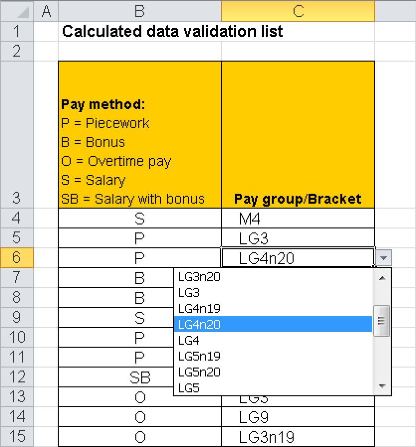
The validation of the pay method in range B4:B15 is straightforward. You need only a fixed entry. In the Data Validation dialog box, click the Settings tab. On the Allow list, select List, and in the Source box, type these options:
P,B,O,S,SBThe validation for the pay group must consider the value in column B. On the Allow list, choose List, and enter the following formula as the source:
=IF(OR($B4="S",$B4="SB"), Salary, Pay)This formula implements the rules (see Table 5-1, shown previously) and displays the applicable list depending on the selected pay method.
If the list option does not provide the flexibility you need, the Custom option offers some further possibilities. When you select Custom on the Allow list in the Data Validation dialog box, you can enter a formula in the Formula box that will return TRUE or FALSE. If the formula returns TRUE, the data is valid. If the formula returns FALSE, the data is invalid and an error message is displayed.
When you use formulas, you have to consider a few limitations in the versions prior to Excel 2007:
You cannot use references to external workbooks, such as the following (see Figure 5-24):
='C:Functions[Workbook.xlsx] Tab1'!$C$3=D7
This is allowed in Excel 2007 and Excel 2010, but the external reference workbook must be open.
You cannot use functions from add-ins. For instance, the NETWORKDAYS() function is only available in a table if the Analysis Functions add-in is installed. This function cannot be used directly for validation.
You cannot use matrix constants.
You cannot use formulas containing more than 255 characters.

To avoid these issues, enter the formula for validation in a table and use a reference to the cell containing the formula for validation.
A common problem with managing lists is duplicate entries. For example, maybe you have to avoid duplicate customer numbers in a customer list, or have to enter each date in a stock price list only once. This can be achieved by using a formula in the validation.
Assume that you want to make sure that each entry the range B2:B20 appears only once. If you try to enter a value more than once, an error message should be displayed.
To set the validation so that each entry can only be used once, do the following:
Select the test range B2:B20.
Open the Data Validation dialog box. On the Settings tab, select Custom on the Allow list.
Add the expression describing the allowed data in the Formula box. To avoid duplicate entries, use this formula (see Figure 5-25):
=COUNTIF($B$2:$B$20,B2)<=1Click the Error Alert tab and enter the error message.
Confirm your entry by clicking OK.
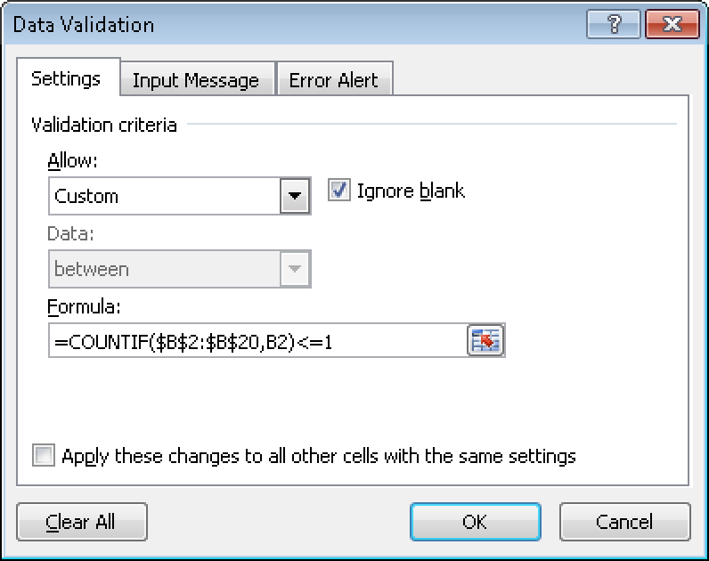
Note that the search range is fixed at $B$2:$B$20, to define the range within which to find duplicates. The second argument of the COUNTIF() function is specified with a relative reference to point to a single input cell. If you look closely at how Excel enters the formula for validation for the range B2:B20, you will see the following:
The search range is always range B2:B20, whereas the Lookup_value always points to the active cell. For this validation, it doesn’t matter if the entry consists of text or numbers. Each entry is checked independently of its data type.
Formulas offer many possibilities. You can monitor a range and display a message after all data entry is complete.
Assume that you want to display a message if all fields in the range B2:B15 are filled out. To view the message when all fields are filled out, do the following:
Select the range B2:B15 and select Data/Validation or click the Data Validation button on the ribbon (in Excel 2007 and Excel 2010).
Choose Custom from the Allow list on the Settings tab, and enter this formula in the Formula field:
=COUNTBLANK($B$2:$B$15)>0Pay attention to the absolute references.
Click the Error Alert tab, and select the Information style.
Enter a title, such as Complete, and enter the text in the Error Message field.
Confirm your entry by clicking OK.
When the last field is entered, a message appears telling the user that the data is complete.