When you’re examining your Excel data to make a business decision, you’ll probably need to look at data from more than one worksheet, or even more than one workbook. Hourly sales totals can help determine when you need more staff on the floor, but if you keep track of the number of customers in the store as well, you might find that your great sales on Monday mornings come from landscape architects loading up for the week. In that case, you would be better off having your warehouse staff and not your counter clerks show up to handle the load.
You can open more than one workbook at a time and arrange them on the screen so you can read data from both sources at the same time. You can do something similar if you have relevant data in two parts of the same worksheet. If you can’t see everything you need to see, you can split the worksheet into two or four units, all with independent scroll bars.
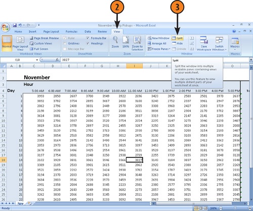
View Different Parts of One Worksheet at the Same Time
Click the cell where you want to split the worksheet.
Click the View tab.
In the Window group, click Split.
Tip
To remove a worksheet split, click the View tab and then, in the Window group, click Split.
Tip
To split a worksheet into two regions instead of four, click the first cell in the row or column where you want to create the split.
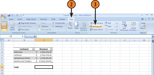
View Multiple Workbooks at the Same Time
Open all the workbooks you want to view.
Click the View tab.
Click Arrange All.
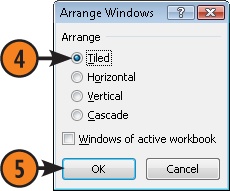
Select the option representing the target arrangement.
Click OK.
Caution
All of the workbooks will now be arranged like this unless you select the Windows Of Active Workbook check box, which will apply the arrangement only to the active workbook.
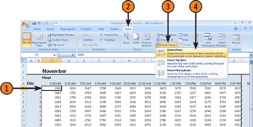
View Multiple Parts of a Worksheet by Freezing Panes
Click the cell below and to the right of where you want to freeze the worksheet.
Click the View tab.
In the Window group, click Freeze Panes.
Click one of the following items:
Freeze Panes, which keeps the cells above or to the left of the current selection visible at all times
Freeze Top Row, which keeps the top row visible at all times
Freeze First Column, which keeps the left-most column visible at all times