
9 Create charts and graphics
In this chapter
Practice files
For this chapter, use the practice files from the Excel2019SBSCh09 folder. For practice file download instructions, see the introduction.
When you enter data into an Excel 2019 worksheet, you create a record of important events, whether they are individual sales, sales for an hour of a day, the price of a product, or something else entirely. What a list of values in cells can’t communicate easily, however, are the overall trends in the data. The best way to communicate trends in a large collection of data is by creating a chart, which summarizes data visually. In addition to standard charts, with Excel 2019 you can create compact charts called sparklines, which summarize a data series by using a graph contained within a single cell.
You have a great deal of control over the appearance of your charts. You can change the color of any chart element, choose a different chart type to better summarize the underlying data, and change the display properties of text and numbers in a chart. If the data in the worksheet used to create a chart represents a progression through time, such as sales over several months, you can have Excel extrapolate future sales and add a trendline to the graph representing that prediction.
This chapter guides you through procedures related to creating charts (including six new chart types in Excel 2019), customizing chart elements, finding trends in your data, summarizing data by using sparklines, creating and formatting diagrams, and creating shapes and mathematical equations.
Create charts
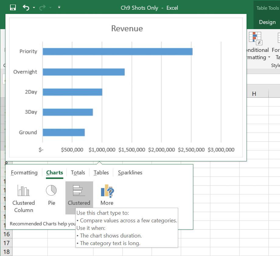
Excel 2019 lets you create charts quickly by using the Quick Analysis Lens, which displays recommended charts to summarize your data. When you select the entire data range you want to chart, clicking the Quick Analysis button that appears in the bottom-right corner of the selection lets you display the types of charts Excel recommends.
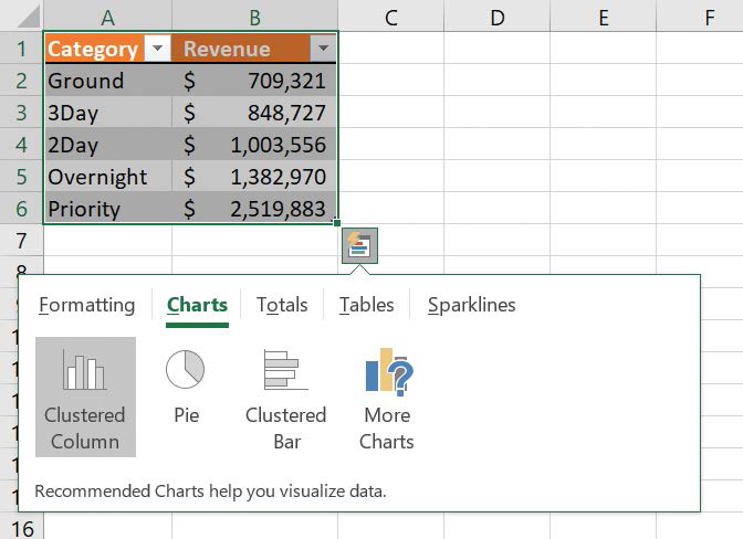
You can display a preview of each recommended chart by pointing to the icon representing that chart. Clicking the icon adds the chart to your worksheet.
![]() Tip
Tip
Press the F11 key to create a chart of the default type on a new chart sheet, which is a distinct type of sheet that only contains a chart and not worksheet cells. Unless you or another user changed the default, Excel creates a column chart.
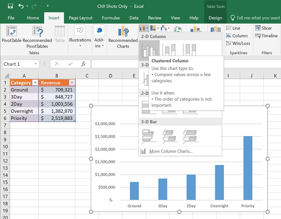
If the chart you want to create doesn’t appear in the list of charts recommended by the Quick Analysis Lens, you can select the chart type you want from a gallery on the Insert tab of the ribbon. When you point to a subtype in the gallery, Excel displays a preview of the chart you will create by clicking that subtype. When you click a chart subtype, Excel creates the chart by using the default layout and color scheme defined in your workbook’s theme.
If Excel doesn’t plot your data the way you want it to, you can change the axis on which Excel plots a data column. The most common reason for incorrect data plotting is that the column to be plotted on the horizontal axis contains numerical data instead of textual data. For example, if your data includes a Year column and a Volume column, instead of plotting volume data for each consecutive year along the horizontal axis, Excel plots both of those columns in the body of the chart and creates a sequential series to provide values for the horizontal axis.
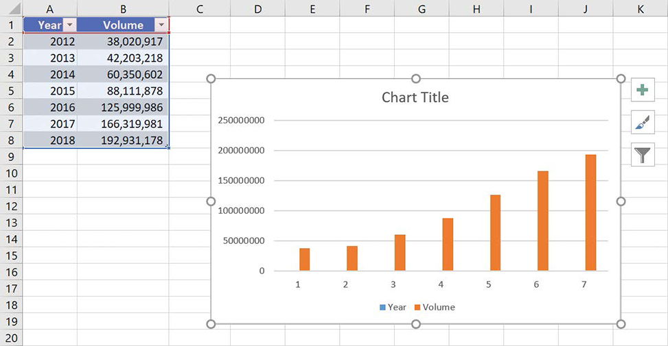
You can change which data Excel applies to the vertical axis (also known as the y-axis) and the horizontal axis (also known as the x-axis). If Excel has swapped the values for the vertical and horizontal axes, you can switch the row and column data to update your chart. If the problem is a little more involved, you can edit how Excel interprets your source data.
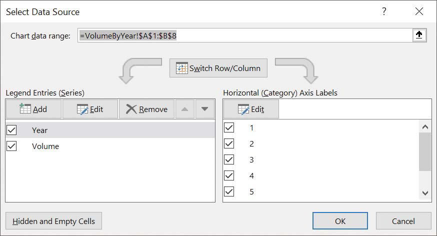
The Year column should appear on the horizontal axis as a data category, which Excel refers to as the axis labels.
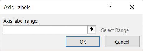
After you identify the cell range that provides the values for your axis labels, Excel will revise your chart.
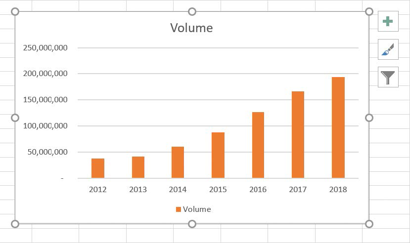
After you create your chart, you can change its size to reflect whether the chart should dominate its worksheet or take on a role as another informative element on the worksheet.
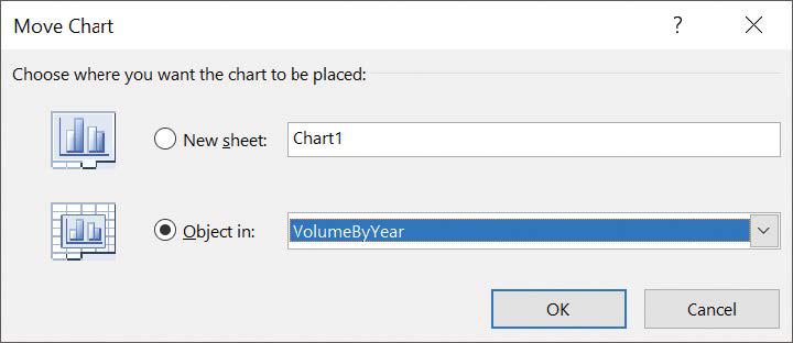
Just as you can control a chart’s size, you can also control its location. You can drag a chart to a new location on its current worksheet, move the chart to another worksheet, or move the chart to its own chart sheet.
To create a chart
Select the data you want to appear in your chart.
On the Insert tab of the ribbon, in the Charts group, click the type and subtype of the chart you want to create.
To create a chart of the default type by using a keyboard shortcut
Select the data you want to summarize in a chart.
Do either of the following:
Press F11 to create the chart on a new chart sheet.
Press Alt+F1 to create the chart on the active worksheet.
To create a chart by using the Quick Analysis Lens
Select the data you want to appear in your chart.
Click the Quick Analysis button.
In the gallery that appears, click the Charts tab.
Click the type of chart you want to create.
To create a recommended chart
Select the data you want to visualize.
On the Insert tab, in the Charts group, click the Recommended Charts button.
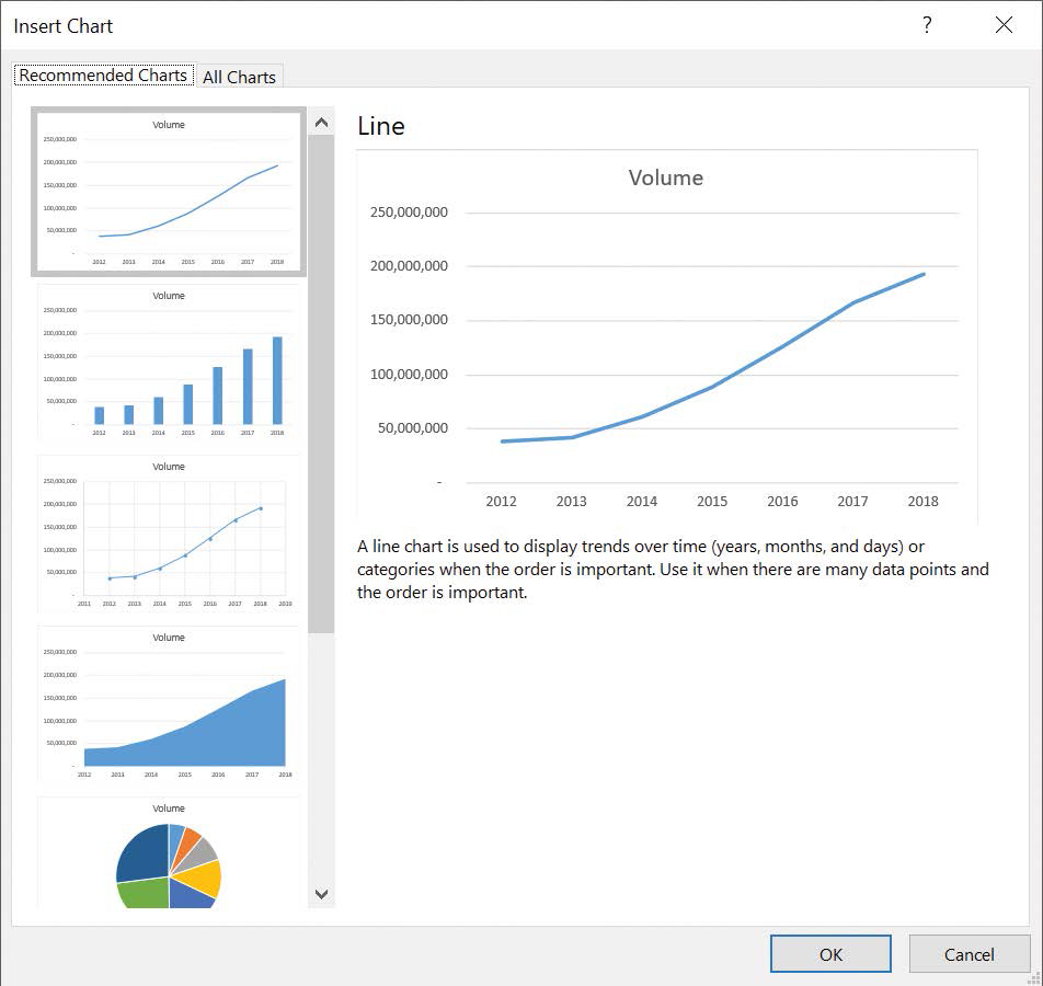
View Excel chart recommendations. In the Insert Chart dialog box, click the chart you want to create.
Click OK.
To change how Excel plots your data in a chart
Click the chart you want to change.
On the Design tool tab of the ribbon, in the Data group, click Select Data.
In the Select Data Source dialog box, do any of the following:
Delete a Legend Entries (Series) data set by clicking the series and clicking the Remove button.
Add a Legend Entries (Series) data set by clicking the Add button and, in the Edit Series dialog box that appears, selecting the cells that contain the data you want to add, and then clicking OK.
Edit a Legend Entries (Series) data set by clicking the series you want to edit, clicking the Edit button, and, in the Edit Series dialog box, selecting the cells that provide values for the series, and then clicking OK.
Change the order of Legend Entries (Series) data sets by clicking the series you want to move and clicking either the Move Up or Move Down button.
Switch the row and column data series by clicking the Switch Row/Column button.
Change the values used to provide Horizontal (Category) Axis Labels by clicking that section’s Edit button and then, in the Axis Labels dialog box that appears, selecting the cells to provide the label values and clicking OK.
To switch row and column values
Click the chart you want to edit.
In the Data group, click the Switch Row/Column button.
To resize a chart
Click the chart you want to edit.
On the Format tool tab, in the Size group, enter new values into the Shape Height and Shape Width boxes.
Or
Drag a handle to change the position of the chart’s edge or corner. You can do any of the following:
Drag the handle in the middle of the top or bottom chart border to change the chart’s height.
Drag a handle in the middle of the left or right chart border to change the chart’s width.
Drag a handle at a corner of the chart border to change both the chart’s height and its width.
To reposition a chart within a worksheet
Click the chart.
Drag it to its new position.
To move a chart to another worksheet
Click the chart.
On the Design tool tab, in the Location group, click the Move Chart button.
In the Move Chart dialog box, click the Object in arrow.
In the Object in list, click the sheet to which you want to move the chart.
Click OK.
To move a chart to its own chart sheet
Click the chart.
In the Location group, click the Move Chart button.
In the Move Chart dialog box, click in the New sheet box.
Enter a name for the new sheet.
Click OK.
Perform business intelligence analysis using charts
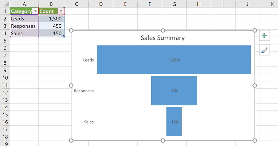
Excel 2019 introduces one new type of chart, the funnel chart, and the ability to create 2D maps of your data. A funnel chart shows how many items in a process continue to the next step. For example, a business might track sales leads, successful contacts, and customers who place an order. The top level of the funnel would depict the leads, the second the successful contacts, and the third customers who placed orders.
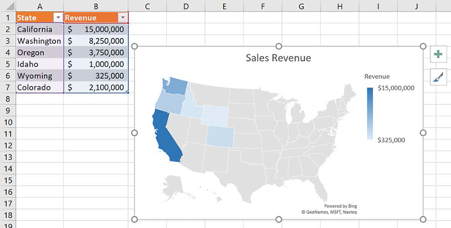
If you collect geographical data, such as your customers’ state of residence, you can summarize that data using a two-dimensional (2D) map. You can mark states from which a customer placed an order or use color or marker size to show the relative number or value of orders from those states.
Excel also includes six types of charts that enhance your ability to analyze and display business data: waterfall, histogram, Pareto, box-and-whisker, treemap, and sunburst. Each of these new chart types enhances your ability to summarize your data and convey meaningful information about your business.
Waterfall charts summarize financial data by distinguishing increases from decreases and indicating whether a particular line item is an individual account, such as Direct Materials, or a broader measure, such as Starting Balance or Ending Balance.
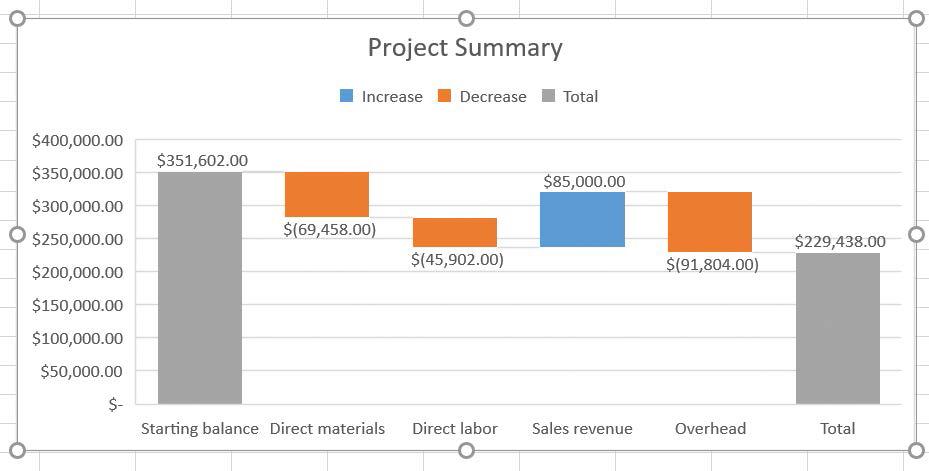
Excel doesn’t automatically recognize which entries should be treated as totals, but you can double-click any columns that represent totals (or subtotals) and identify them so Excel knows how to handle them.
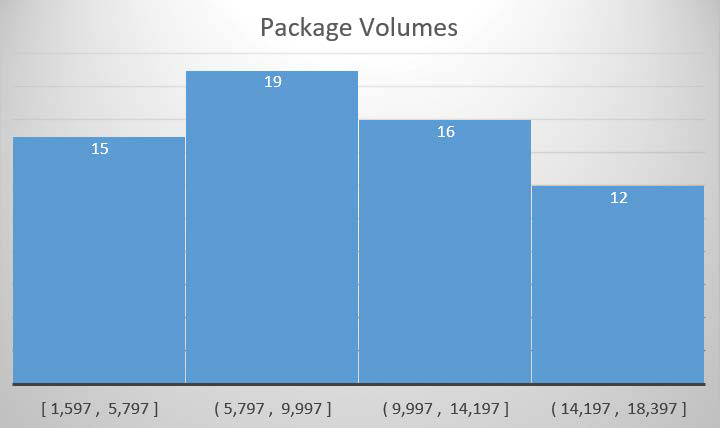
Histograms count the number of occurrences of values within a set of ranges, where each range is called a bin. For example, a summary of daily package volumes for a delivery area could fall into several ranges.
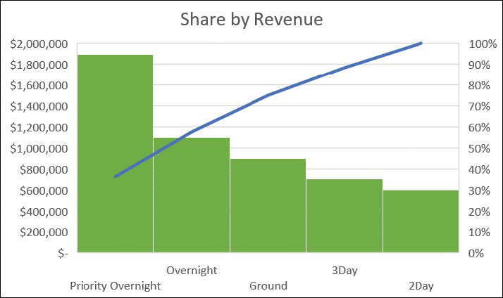
A Pareto chart combines a histogram and a line chart to show both the contributions of categories of values, such as package delivery options (for example, overnight, priority overnight, and ground), and the cumulative contributions after each category is counted.
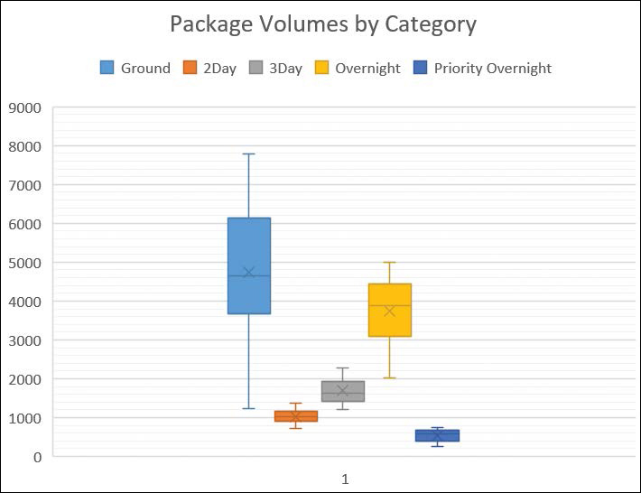
A box-and-whisker chart combines several statistical measures, including the average (or mean), median, minimum, and maximum values for a data series, into a single chart. These charts provide a compact yet informative view of your data from a statistical standpoint.
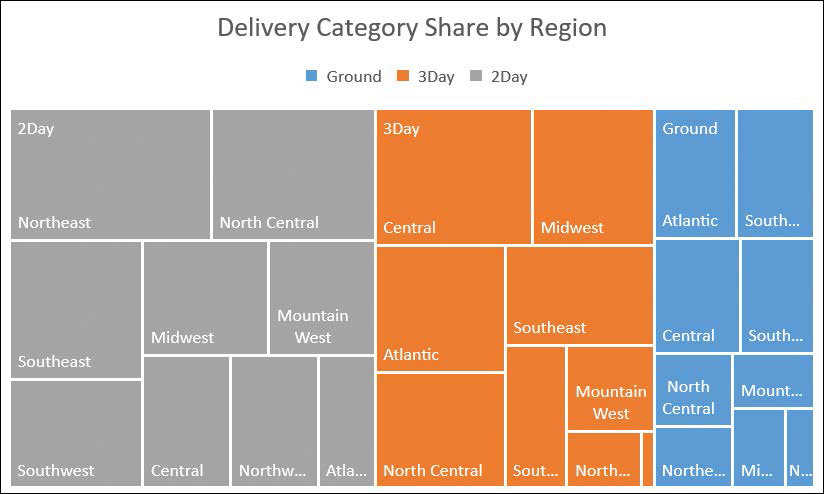
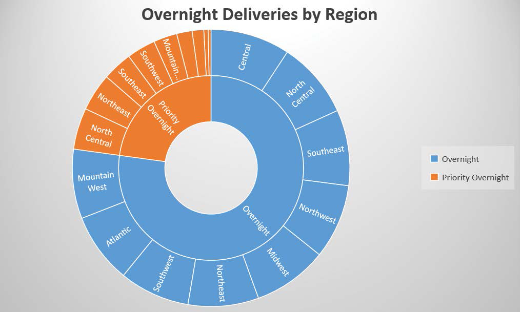
The treemap chart divides data into categories, which are represented by colors, and shows the hierarchy of values within each category by using the size of the rectangles within the category. For example, you could represent regional frequencies for each package delivery option available to customers.
A sunburst chart breaks down a data set’s hierarchy to an even deeper level, showing the details of how much each subcategory of data contributes to the whole.
To create a funnel chart
Select the data you want to visualize.
On the Insert tab, in the Charts group, click the Insert Waterfall, Funnel, Stock, Surface, or Radar Chart button.
In the Funnel group, click the Funnel chart type.
To create a 2D map chart
Select the data you want to visualize.
On the Insert tab, in the Charts group, click the Maps button, and then click the Filled Map chart type.
If necessary, give Excel permission to upload your data to Bing Maps to create the chart.
 Important
If you attempt to map data that does not include an identifiable geographic element, Excel displays an error message. If that error occurs, verify the data range you selected.
To create a waterfall chart
Select the data you want to visualize.
On the Insert tab, in the Charts group, click the Insert Waterfall, Funnel, Stock, Surface, or Radar Chart button.
Click the Waterfall chart type.
If necessary, identify a column as a total by clicking the column once to select the series, clicking the column again to select it individually, right-clicking the column, and then clicking Set as Total.
To create a histogram chart
Select the data you want to visualize.
In the Charts group, click the Insert Statistic Chart button.
In the Histogram group, click the Histogram subtype.
To create a Pareto chart
Select the data you want to visualize.
Click the Insert Statistic Chart button.
In the Histogram group, click the Pareto subtype.
To create a box-and-whisker chart
Select the data you want to visualize.
Click the Insert Statistic Chart button.
In the Histogram group, click the Box and Whisker subtype.
To create a treemap chart
Select the data you want to visualize.
In the Charts group, click the Insert Hierarchy Chart button.
In the Treemap group, click the Treemap subtype.
To create a sunburst chart
Select the data you want to visualize.
Click the Insert Hierarchy Chart button.
In the Sunburst group, click the Sunburst subtype.
Customize chart appearance
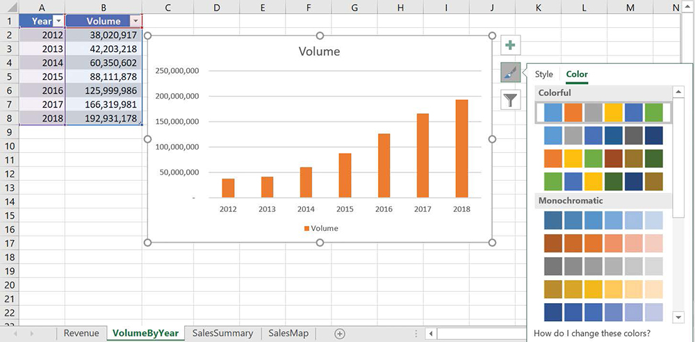
If you want to change a chart’s appearance, you can do so by using the Chart Styles button, which appears in a group of three buttons next to a selected chart. These buttons put chart formatting and data controls within easy reach.
Clicking the Chart Styles button opens a gallery that has two tabs: Style and Color. The Style tab contains 14 styles from which to choose, and the Color tab displays a series of color schemes you can select to change your chart’s appearance.
![]() Tip
Tip
If you prefer to work with the ribbon, these same styles appear in the Chart Styles gallery on the Design tab.
![]() Tip
Tip
The colors and styles in the Chart Styles gallery are tied to your workbook’s theme. If you change your workbook’s theme, Excel changes the colors available in the Chart Styles gallery, as well as your chart’s appearance, to reflect the new theme’s colors.
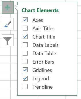
When you create a chart, Excel creates a visualization that focuses on the data. In most cases, the chart has a title, a legend (a list of the data series displayed in the chart), horizontal lines in the body of the chart to make it easier to discern individual values, and axis labels. If you want to create a chart that has more or different elements, such as additional data labels for each data point plotted on your chart, you can do so by selecting a new layout. If it’s still not quite right, you can show or hide individual elements by using the Chart Elements button.
After you select a chart element, you can change its size and appearance by using controls specifically created to work with that element type.
You can use the third button, Chart Filters, to focus on specific data in your chart. Clicking the Chart Filters button displays a filter interface that is very similar to that used to limit the data displayed in an Excel table.
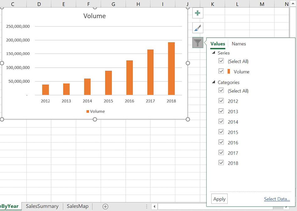
Selecting or clearing a check box displays or hides data related to a specific value within a series. You can also use the check boxes in the Series section of the panel to display or hide entire data series.
If you think you want to apply the same set of changes to charts you’ll create in the future, you can save your chart as a chart template. When you select the data you want to summarize visually and apply the chart template, you’ll create consistently formatted charts in a minimum of steps.
To apply a built-in chart style
Click the chart you want to format.
On the Design tool tab, in the Chart Styles gallery, click the style you want to apply.
Or
Click the chart you want to format.
Click the Chart Styles button.
If necessary, click the Style tab.
Click the style you want to apply.
To apply a built-in chart layout
Click the chart you want to format.
In the Chart Layouts group, click the Quick Layout button.
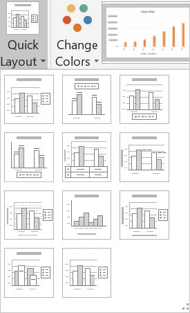
Select a new layout from the Quick Layout gallery. Click the layout you want to apply.
To change a chart’s color scheme
Click the chart you want to format.
In the Chart Styles group, click the Change Colors button.
Click the color scheme you want to apply.
Or
Click the chart you want to format.
Click the Chart Styles button.
If necessary, click the Color tab.
Click the color scheme you want to apply.
To select a chart element
Click the chart element.
Or
Click the chart.
On the Format tool tab, in the Current Selection group, click the Chart Elements arrow.
Click the chart element you want to select.
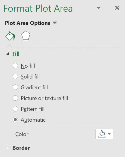
To format a chart element
Select the chart element.
Use the tools on the Format tool tab to change the element’s formatting.
Or
In the Current Selection group, click the Format Selection button to display the Format Chart Element task pane.
Change the element’s formatting.
To display or hide a chart element
Click the chart and do either of the following:
On the Design tool tab, in the Chart Layouts group, click the Add Chart Element button, point to the element on the list, and click None to hide the element, or click one of the other options to show the element.
Click the Chart Elements button and select or clear the check box next to the element you want to show or hide.
To create a chart filter
Click the chart you want to filter.
Click the Chart Filters button.
Use the tools on the Values and Names tabs to create your filter.
To save a chart as a chart template
Right-click the chart.
Click Save as Template.
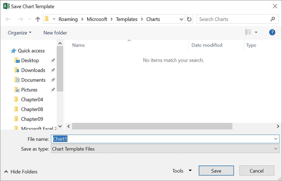
Save a chart as a template so that you can apply consistent formatting quickly. In the File name box, enter a name for the template.
Click Save.
To apply a chart template
Click the chart to which you want to apply a template.
On the Design tool tab, in the Type group, click Change Chart Type.
If necessary, click the All Charts tab.
Click the Templates category.
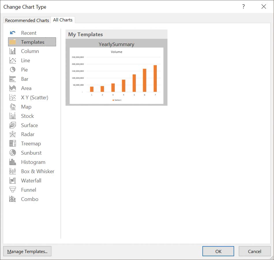
Apply a chart template to give your charts a consistent appearance. Click the template you want to apply.
Click OK.
Find trends in your data
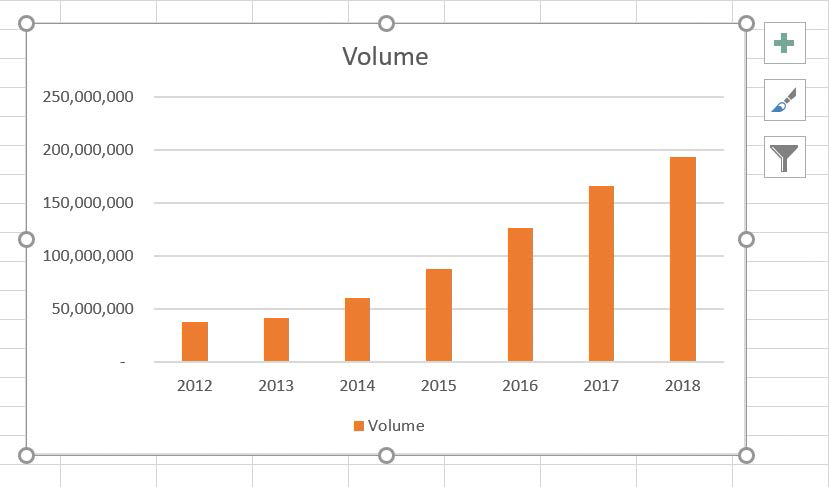
You can use the data in Excel workbooks to discover how your business has performed in the past, but you can also have Excel 2019 make its best guess, for example, as to future shipping revenues if the current trend continues. As an example, consider a line chart that shows package volume data for the years 2012 through 2018.
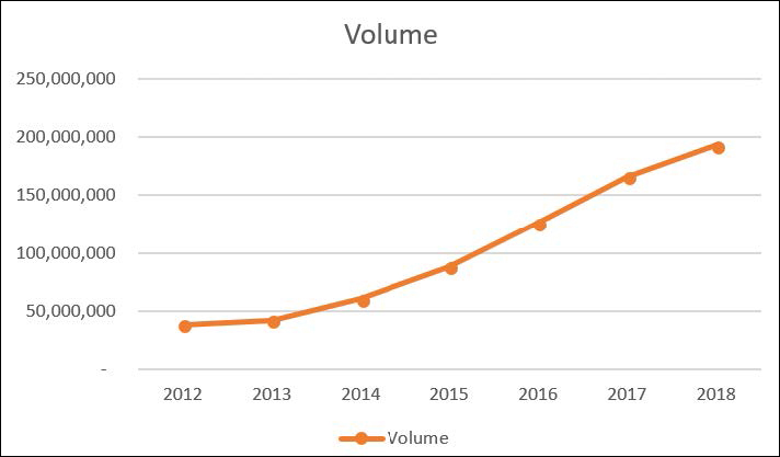
The total has increased from 2012 to 2018, but the growth hasn’t been uniform, so guessing how much package volume would increase if the overall trend continued would require detailed mathematical computations. Fortunately, Excel knows that math and can use it to add a trendline to your data.
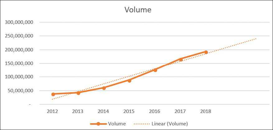
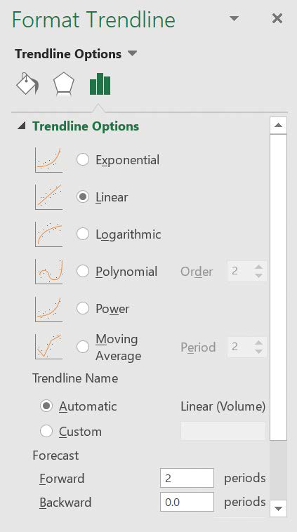
You can choose the data distribution that Excel should expect when it makes its projection. The right choice for most business data is Linear; other distributions (such as Exponential, Logarithmic, and Polynomial) are used for scientific and operations research applications. You can also tell how far ahead Excel should look. Looking ahead by zero periods shows the best-fit line for the current data set, whereas looking ahead two periods would project two periods into the future, assuming current trends continue.
![]() Tip
Tip
When you select a chart, click the Chart Elements button, and click the right-pointing triangle beside Trendline, one of the options Excel displays is Linear Forecast, which adds a trendline with a two-period forecast.
As with other chart elements, you can double-click the trendline to open a formatting dialog box and change the line’s appearance.
To add a trendline to a chart
Click the chart to which you want to add a trendline.
On the Design tool tab, in the Chart Layouts group, click the Add Chart Element button.
Point to Trendline and click the type of trendline you want to add.
To edit a trendline’s properties and appearance
Click the chart that contains the trendline.
On the Format tool tab, in the Current Selection group, click the Chart Elements arrow.
Click the element that ends with the word Trendline.
Click Format Selection.
Use the controls in the Format Trendline task pane to edit the trendline’s properties and appearance.
To delete a trendline
Click the trendline.
Press the Delete key.
Create combo charts
The Excel 2019 charting engine is powerful, but it does have its quirks. Some data collections you might want to summarize in Excel will have more than one value related to each category. For example, each regional center for a package-delivery company could have both overall package volume and revenue for the year. You can restructure the data in your Excel table to create a combo chart, which uses two vertical axes to show both value sets in the same chart.
![]() Tip
Tip
A Pareto chart, discussed earlier in this chapter, is a type of dual-axis chart.
To create a dual-axis chart
Select the data you want to visualize.
On the Insert tab, in the Charts group, click the Insert Combo Chart button.
Click the type of combo chart you want to create.
Or
Click Create Custom Combo Chart and use the settings in the Combo category of the All Charts tab to define your combo chart.
Summarize your data by using sparklines
You can create charts in Excel to summarize your data visually by using legends, labels, and colors to highlight aspects of your data. It is possible to create very small charts to summarize your data in an overview worksheet, but you can also use a sparkline to create a compact, informative chart that provides valuable context for your data.
Edward Tufte introduced sparklines in his book Beautiful Evidence (Graphics Press, 2006), with the goal of creating charts that imparted their information in approximately the same space as a word of printed text. In Excel, a sparkline occupies a single cell, which makes it ideal for use in summary worksheets.
You can create three types of sparklines: line, column, and win/loss. The line and column sparklines are compact versions of the standard line and column charts. The win/loss sparkline indicates whether a cell value is positive (a win), negative (a loss), or zero (a tie).
After you create a sparkline, you can change its appearance. Because a sparkline takes up the entire interior of a single cell, resizing that cell’s row or column resizes the sparkline. You can also change a sparkline’s formatting, modify its labels, or delete it entirely.
![]() Tip
Tip
Sparklines work best when displayed in compact form. If you find yourself adding markers and labels to a sparkline, you might consider using a regular chart to take advantage of its wider range of formatting and customization options.
To create a sparkline
Select the data you want to visualize.
On the Insert tab, in the Sparklines group, do one of the following:
Click the Line button.
Click the Column button.
Click the Win/Loss button.
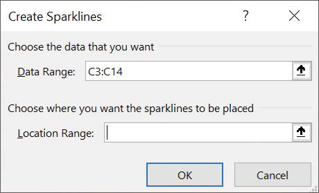
Insert a sparkline by using the Create Sparklines dialog box. In the Create Sparklines dialog box, verify that the data you selected appears in the Data Range box.
If the wrong data appears, click the Collapse Dialog button next to the Data Range box, select the cells that contain your data, and then click the Expand Dialog button.
Click the Collapse Dialog button next to the Location Range box, click the cell where you want the sparkline to appear, and then click the Expand Dialog button.
Click OK.
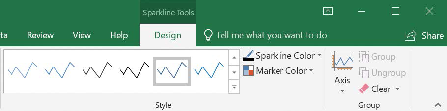
To format a sparkline
Click the cell that contains the sparkline.
Use the tools on the Design tool tab to format the sparkline.
To delete a sparkline
Click the cell that contains the sparkline.
On the Design tool tab, in the Group group, click the Clear button.
Create diagrams by using SmartArt
Businesses define processes to manage product development, sales, and other essential functions. Excel 2019 comes with a selection of built-in diagram types, referred to as SmartArt, that you can use to illustrate processes, lists, and hierarchies within your organization.
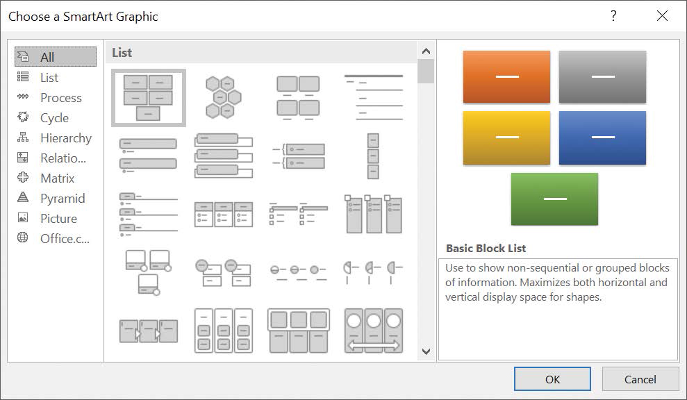
Clicking one of the buttons in the dialog box selects the type of diagram the button represents and causes a description of the diagram type to appear in the rightmost pane of the dialog box. The following table lists the nine categories of diagrams from which you can choose.
Diagram |
Description |
|---|---|
List |
Shows a series of items that typically require a large amount of text to explain |
Process |
Shows a progression of sequential steps through a task, process, or workflow |
Cycle |
Shows a process with a continuous cycle or relationships of core elements |
Hierarchy |
Shows hierarchical relationships, such as those within a company |
Relationship |
Shows the relationship between two or more items |
Matrix |
Shows the relationship of components to a whole by using quadrants |
Pyramid |
Shows proportional, foundation-based, or hierarchical relationships such as a series of skills |
Picture |
Shows one or more images with captions |
Office.com |
Shows diagrams available from Office.com |
![]() Tip
Tip
Some of the diagram types can be used to illustrate several types of relationships. Be sure to examine all your options before you decide on the type of diagram to use to illustrate your point.
After you click the button representing the type of diagram you want to create, clicking OK adds the diagram to your worksheet. As with other drawing objects and shapes, you can move, copy, and delete the SmartArt diagram as needed.
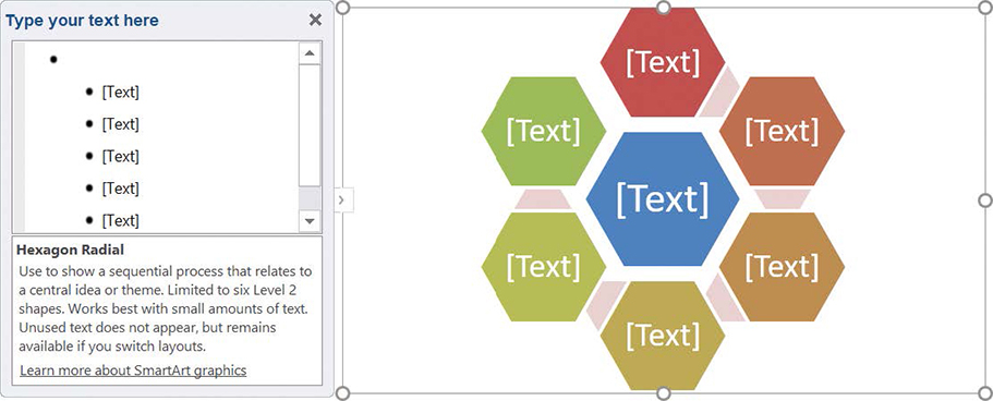
While the diagram is selected, you can add and edit text; add, edit, or reposition shapes; and use the buttons on the ribbon to change the shapes’ formatting. To add text, you can either type directly into the shape or use the Text Pane, which appears beside the SmartArt diagram. When you’re done, click outside the shape to stop editing.
![]() Tip
Tip
Pressing the Enter key after you edit the text in a SmartArt shape adds a new shape to the diagram.
To create a SmartArt graphic
Display the worksheet where you want the SmartArt graphic to appear.
On the Insert tab, in the Illustrations group, click the SmartArt button.
In the Choose a SmartArt Graphic dialog box, click the category from which you want to choose your graphic style.
Click the style of graphic you want to create.
Click OK.
To edit text in a SmartArt graphic shape
Click the shape, and then do either of the following:
Edit the text directly in the shape.
Click the corresponding line in the Type Your Text Here pane and edit the text there.
To format shape text
Click the shape that contains the text you want to format.
Use the tools on the mini toolbar or the Home tab of the ribbon to format the text.
To add a shape
Click the shape next to where you want the new shape to appear.
On the Design tool tab, in the Create Graphic group, click the Add Shape arrow (not the button) and select where you want the new shape to appear.
 Tip
TipIf you click the Add Shape button (not the arrow), Excel adds a shape below or to the left of the current shape.
To delete a shape
Click the shape.
Press Delete.
To change a shape’s position
Click the shape you want to move.
In the Create Graphic group, do either of the following:
Click Move Up.
Click Move Down.
To change a shape’s level
Click the shape you want to move.
In the Create Graphic group, do either of the following:
Click Promote.
Click Demote.
To change a SmartArt graphic’s layout
Click the SmartArt graphic.
On the Design tool tab, in the Layouts group, click the More button in the lower-right corner of the Layouts gallery.
Select a new layout for your SmartArt diagram. Click the new layout.
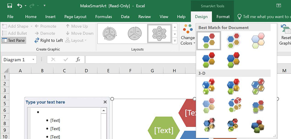
To change a SmartArt graphic’s color scheme
Click the SmartArt graphic.
On the Design tool tab, in the SmartArt Styles group, click the Change Colors button and click a new color scheme.
To apply a SmartArt Style
Click the SmartArt graphic.
In the SmartArt Styles group, click the More button in the lower-right corner of the SmartArt Styles gallery, and click the style you want to apply.
To format a shape
Click the shape you want to format.
Use the tools on the Format tool tab to change the shape’s formatting.
To delete a SmartArt diagram
Right-click the diagram, and then click Cut.
Create and manage shapes
With Excel, you can analyze your worksheet data in many ways, including summarizing your data and business processes visually by using charts and SmartArt. You can also augment your worksheets by adding objects such as geometric shapes, lines, flowchart symbols, and banners.
![]() Tip
Tip
A SmartArt diagram is a collection of shapes that Excel treats as a collective unit. The shapes described in this topic are individual objects that Excel manages independently.
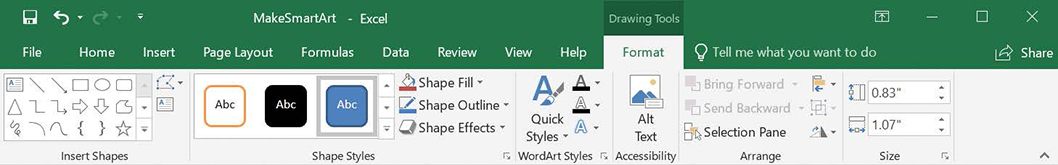
After you draw a shape on a worksheet, or select it after you’ve drawn it, you can use the controls on the Format tool tab of the ribbon to change its appearance.
![]() Tip
Tip
Holding down the Shift key while you draw a shape keeps the shape’s height, width, and other characteristics equal. For example, clicking the Rectangle tool and then holding down the Shift key while you draw the shape causes you to draw a square.
You can resize a shape by clicking the shape and then dragging one of the resizing handles that appears around the edge of the shape. You can drag a handle on a side of the shape to drag that side to a new position; if you drag a handle on the corner of the shape, you affect height and width simultaneously. If you hold down the Shift key while you drag a shape’s corner, Excel keeps the shape’s height and width in proportion as you drag the corner. You can also rotate a shape until it is in the orientation you want.
![]() Tip
Tip
You can assign your shape a specific height and width by clicking the shape and then, on the Format tool tab, in the Size group, entering the values you want in the Shape Height and Shape Width boxes.
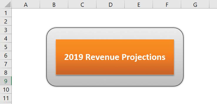
After you create a shape, you can use the controls on the Format tool tab to change its formatting. You can apply predefined styles or use the options accessible from the Shape Fill, Shape Outline, and Shape Effects buttons to change those aspects of the shape’s appearance.
![]() Tip
Tip
When you point to a formatting option, such as a style or option displayed in the Shape Fill, Shape Outline, or Shape Effects lists, Excel displays a live preview of how your shape would appear if you applied that formatting option. You can preview as many options as you want before committing to a change.
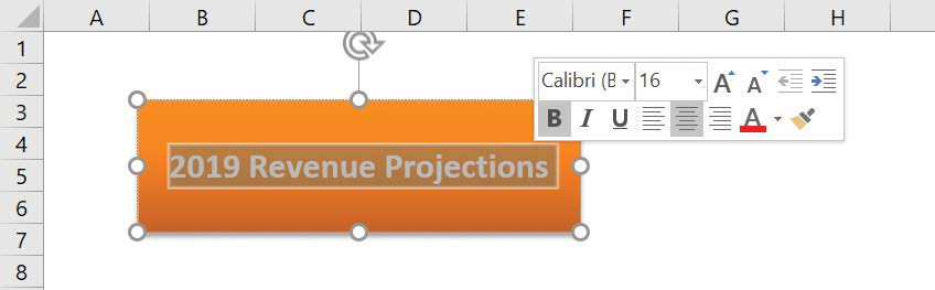
If you want to use a shape as a label or header in a worksheet, you can add text to the shape’s interior by clicking the shape and typing. If you want to edit a shape’s text, point to the text. When the mouse pointer is in position, it will change from a white pointer with a four-pointed arrow to a black I-bar. You can then click the text to start editing it or change its formatting.
You can move a shape within your worksheet by dragging it to a new position. If your worksheet contains multiple shapes, you can align and distribute them within the worksheet. Aligning shapes horizontally means arranging them so they are lined up by their top edge, bottom edge, or horizontal center. Aligning them vertically means lining them up so that they have the same right edge, left edge, or vertical center. Distributing shapes moves the shapes so they have a consistent horizontal or vertical distance between them.
If you have multiple shapes on a worksheet, you will find that Excel arranges them from front to back, placing newer shapes in front of older shapes.
You can change the order of the shapes to create exactly the arrangement you want, whether by moving a shape one step forward or backward, or by moving it all the way to the front or back of the stack.
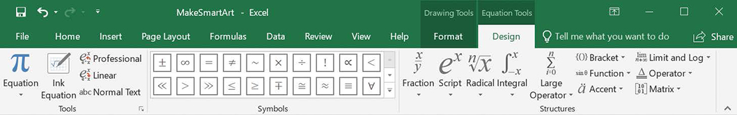
Create and manage mathematical equations
One other way to enhance your Excel files is to add mathematical equations to a worksheet. You can create a wide range of formulas by using built-in structures and symbols.
![]() Tip
Tip
Clicking the arrow at the bottom of the Equation button at the left end of the Equation Tools tab displays a list of common equations, such as the Pythagorean Theorem, that you can add with a single click.
Excel 2019 also provides the new capability of interpreting a handwritten equation that you draw directly into your worksheet.

To add a shape to a worksheet
On the Insert tab, in the Illustrations group, click the Shapes button to display the Shapes list.
Click the shape you want to add.
Click and drag in the body of the worksheet to define the shape.
To move a shape
Click the shape and drag it to its new location.
To resize a shape
Do either of the following:
Grab a handle on an edge or corner of the shape and drag inward or outward to move one or more edges.
On the Format tool tab, in the Size group, enter new values in the Shape Height and Shape Width boxes.
To rotate a shape
Click the shape and do one of the following:
Drag the rotate handle (it looks like a clockwise-pointing circular arrow) above the shape to a new position.
On the Format tool tab, in the Arrange group, click the Rotate button, and then select the rotate option you want.
Click the Rotate button, and then click More Rotation Options to use the tools in the Format Shape task pane.
To change shape formatting
Click the shape you want to format.
Use the tools on the Format tool tab to change the shape’s appearance.
To add text to a shape
Click the shape.
Enter the text you want to appear in the shape.
Click outside the shape to stop editing its text.
To edit shape text
Point to the text in the shape. When the mouse pointer changes to a thin I-bar, click once.
Edit the shape’s text.
Click outside the shape to stop editing its text.
To format shape text
Point to the text in the shape. When the mouse pointer changes to a thin I-bar, click once.
Select the text you want to edit.
Use the tools on the mini toolbar and the Home tab of the ribbon to format the text.
Click outside the shape to stop editing its text.
To align shapes
Select the shapes you want to align.
On the Format tool tab, in the Arrange group, click the Align button.
Click the alignment option you want to apply to your shapes.
To distribute shapes
Select three or more shapes.
Click the Align button, and do either of the following:
Click Distribute Horizontally to place the shapes on the worksheet with evenly spaced horizontal gaps between them.
Click Distribute Vertically to place the shapes on the worksheet with evenly spaced vertical gaps between them.
To reorder shapes
Click the shape you want to move.
In the Arrange group, do either of the following:
Click the Bring Forward arrow, and then click Bring Forward or Bring to Front.
Click the Send Backward arrow, and then click Send Backward or Send to Back.
To delete a shape
Click the shape.
Press Delete.
To add a preset equation to a worksheet
On the Insert tab, in the Symbols group, click the Equation arrow (not the button).
Click the equation you want to add.
To add an equation to a worksheet
In the Symbols group, click the Equation button.
Use the tools on the Design tool tab of the ribbon to create the equation.
To add a handwritten equation to a worksheet
Click the Equation arrow.
Click Ink Equation.
In the Write Math Here area, write the equation you want to enter.
Click Insert.
To edit an equation
Click the part of the equation you want to edit.
Enter new values for the equation.
To delete an equation
Click the edge of the equation’s shape to select it.
Press Delete.
Skills review
In this chapter, you learned how to:
Create charts
Perform business intelligence analysis using charts
Customize chart appearance
Find trends in your data
Create combo charts
Summarize your data by using sparklines
Create diagrams by using SmartArt
Create and manage shapes
Create and manage mathematical equations
Practice tasks

The practice files for these tasks are located in the Excel2019SBSCh09 folder. You can save the results of the tasks in the same folder.
Create charts
Open the CreateCharts workbook in Excel, and then perform the following tasks:
Using the values on the Data worksheet, create a column chart.
Change the column chart so it uses the Year values in cells A3:A9 as the horizontal (category) axis values, and the Volume values in cells B3:B9 as the vertical axis values.
Using the same set of values, create a line chart.
Using the Quick Analysis Lens, create a pie chart from the same data.
Perform business intelligence analysis using charts
Open the CreateNewCharts workbook in Excel, and then perform the following tasks:
Use the data on the Funnel worksheet to create a funnel chart.
Use the data on the Mapping worksheet to create a 2D map by state.
Use the data on the Waterfall worksheet to create a waterfall chart. Identify the Starting Balance and Total values as totals.
Use the data on the Histogram worksheet to create a histogram.
Use the data on the Pareto worksheet to create a Pareto chart.
Use the data on the BoxAndWhisker worksheet to create a box-and-whisker chart.
Use the data on the Treemap worksheet to create a treemap chart.
Use the data on the Sunburst worksheet to create a sunburst chart.
Customize chart appearance
Open the CustomizeCharts workbook in Excel, and then perform the following tasks:
Using the chart on the Presentation worksheet, change the chart’s color scheme.
Change the same chart’s layout.
Using the chart on the Yearly Summary worksheet, change the chart’s type to a line chart.
Move the chart on the Yearly Summary worksheet to a new chart sheet.
Find trends in your data
Open the IdentifyTrends workbook in Excel, and then perform the following tasks:
Using the chart on the Data worksheet, add a linear trendline that draws the best-fit line through the existing data.
Edit the trendline so it shows a forecast two periods into the future.
Delete the trendline.
Create combo charts
Open the MakeComboCharts workbook in Excel, and then perform the following tasks:
Using the data on the Summary worksheet, create a dual-axis chart that displays the Volume series as a column chart and the Exceptions series as a line chart.
Ensure that the Exceptions values are plotted on the minor vertical axis at the right edge of the chart.
Summarize your data by using sparklines
Open the CreateSparklines workbook in Excel, and then perform the following tasks:
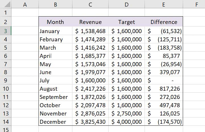
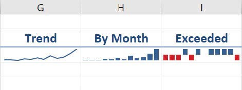
Using the data in cells C3:C14, create a line sparkline in cell G3.
Using the data in cells C3:C14, create a column sparkline in cell H3.
Using the data in cells E3:E14, create a win/loss sparkline in cell I3.
Change the color scheme of the win/loss sparkline.
Delete the sparkline in cell H3.
Create diagrams by using SmartArt
Open the MakeSmartArt workbook in Excel, and then perform the following tasks:
Create a process SmartArt diagram.
Fill in the shapes with the steps for a process with which you’re familiar.
Add a shape to the process.
Change the place where one of the shapes appears in the diagram.
Change the diagram’s color scheme.
Delete a shape from the diagram.
Create and manage shapes and mathematical equations
Open the CreateShapes workbook in Excel, and then perform the following tasks:
Create three shapes and add text to each of them.
Edit and format the text in one of the shapes.
Move the shapes so you can determine which is in front, which is in the middle, and which is in back.
Change the shapes’ order and observe how it changes the appearance of the worksheet.
Align the shapes so their middles are on the same line.
Distribute the shapes evenly in the horizontal direction.
Delete one of the shapes.
Create and manage mathematical equations
Open the CreateEquations workbook in Excel, and then perform the following tasks:
Add a built-in equation such as the quadratic formula.
Enter an equation manually.