
15 Perform business intelligence analysis
In this chapter
Practice files
For this chapter, use the practice files from the Excel2019SBSCh15 folder. For practice file download instructions, see the introduction.
Organizations of all kinds generate and collect data from operations, sales, and customers. As the volume of data grows, so does the importance of generating useful insights into your operations from that data. Excel supports business intelligence analysis, which is the practice of examining data to improve business performance.
Analytical tools such as formulas, data tables, and PivotTables all provide valuable insights into your data, but their applications can be limited in size and scope. Excel 2019 includes many advanced data analysis capabilities that were previously exclusive to enterprise customers. One technology underlying the new tools is the Excel Data Model, which you can use to create relationships among Excel tables in your workbooks. Add to this the ability to import and analyze large data sets by using Power Query and Power Pivot, and Excel 2019 puts significant data analysis capabilities at your fingertips.
This chapter guides you through procedures related to enabling the Data Analysis add-ins and adding tables to the Data Model, defining relationships between tables, analyzing data by using Power Pivot, viewing data by using timelines, and bringing in external data by using Power Query.
![]() Important
Important
The tools and techniques described in this chapter will be available to you only after you enable the Data Analysis add-ins.
Define a Data Model
Excel 2019 includes a collection of Data Analysis add-ins you can use to perform advanced analysis on your data. These tools build on the Excel Data Model, which manages Excel tables, query tables, and other data sources, as part of a coherent whole, rather than individual tables.
After you enable the Data Analysis add-ins, you can add data sources to the Data Model, display the Data Model, and return to your main Excel workbook.
To enable the Data Analysis add-ins
Display the Backstage view, and then click Options.
In the Excel Options dialog box, click Data.
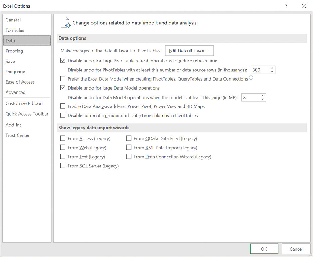
Enable the Data Analysis add-ins from the Excel Options dialog box. In the Data options group, select the Enable Data Analysis add-ins: Power Pivot, Power View and 3D Maps check box.
Click OK.
To add an Excel table to the Data Model
If necessary, enable the Data Analysis add-ins.
Click any cell in the Excel table.
On the Power Pivot tab, in the Tables group, click Add to Data Model to add the Excel table and display it in the Power Pivot window.
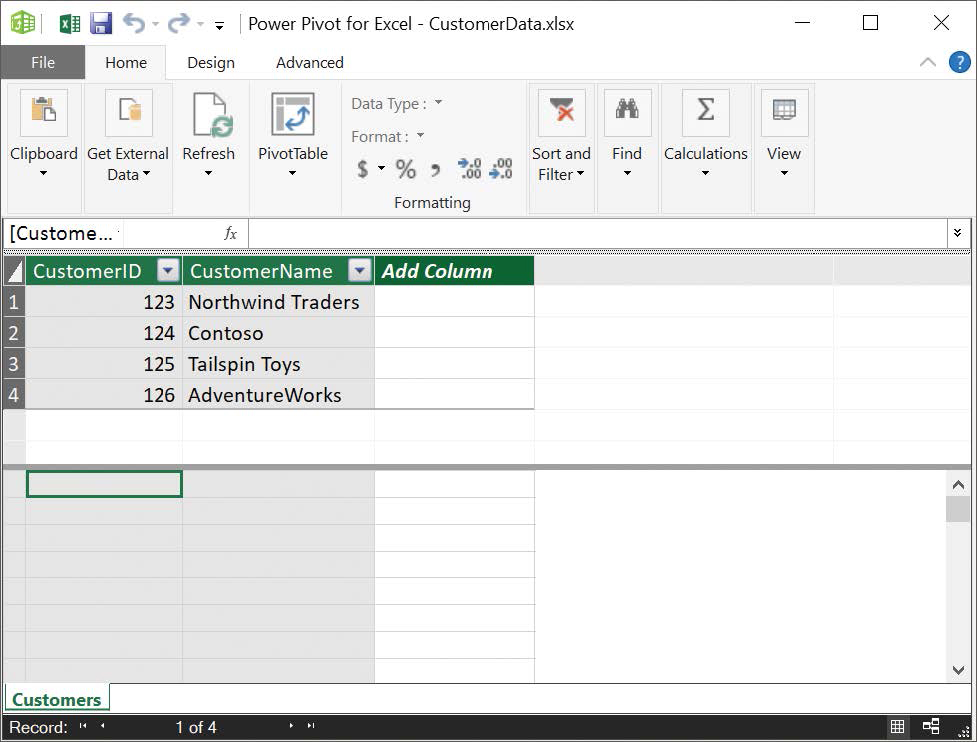
View of the Data Model after an Excel table has been added.
To set a preference to add data to the Data Model
Open the Excel Options dialog box, and then click Advanced.
In the Data group, select the Prefer the Data Model when creating PivotTables, QueryTables, and Data Connections check box.
Click OK.
To display the Data Model
On the Data tab, in the Data Tools group, click Manage Data Model.
Or
On the Power Pivot tab, in the Data Model group, click Manage.
In the Power Pivot for Excel window, on the tab bar, click the sheet tab of the worksheet you want to display.
To return to the Excel workbook
Perform either of these actions:
In the Power Pivot for Excel window, click the Close button to close Power Pivot and return to Excel.
On the title bar of the Power Pivot for Excel window, click Switch to Workbook to return to Excel without closing Power Pivot.
Define relationships between tables
One of the fundamental principles of good database design is to store data about specific business objects, such as customers, products, or orders, in a table by itself, separate from the other tables in the database. For example, you might store data about customers in one table and data about shipments in another.
Each table has one column, or field, that contains a unique value for each row. This type of column, called a key, makes it possible to distinguish a row from every other row. For example, a table listing customers could have a CustomerID field as its key, with the same field appearing in a table named Orders, which tracks the date, time, value, and identity of the customer who placed each order.
![]() Tip
Tip
The best keys are arbitrary numerical values. If you try to store information in a key field, you will likely run into issues of duplication that make processing your data harder, not easier.
You can create connections between tables by identifying fields they have in common. For example, consider a Customers table that has two fields—CustomerID and CustomerName—and an Orders table that has three fields—OrderID, CustomerID, and OrderPrice. The CustomerID field appears in both tables, so it can be used to establish a link, or relationship.
![]() Important
Important
You must add Excel tables to the Data Model to define relationships between them.
In the Customers table, each CustomerID field value occurs exactly once, so that column is called a primary key. The CustomerID field also occurs in the Orders table, but because it’s possible for a customer to place more than one order, the CustomerID field’s values can repeat. When a key field appears in another table in which it doesn’t distinguish each row from every other row, it’s called a foreign key.
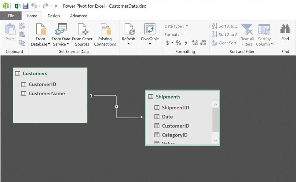
When you create a relationship, you link the primary key field from one table to the corresponding foreign key field in another table. Although it’s easier to spot the fields if they have the same name, such as CustomerID, they don’t have to have the same name; they just need to contain the same data.
After you define a relationship in the Data Model, you can create PivotTables that use data from both Excel tables. You can also edit or delete relationships if necessary.
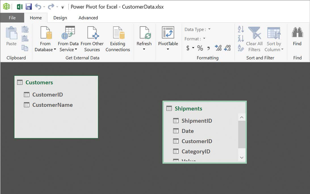
To display the Data Model in Diagram View
If necessary, on the Data tab, in the Data Tools group, click Manage Data Model.
In the Power Pivot for Excel window, on the Home tab, in the View group, click Diagram View.
To display the Data Model in Data View
If necessary, click Manage Data Model.
In the Power Pivot for Excel window, in the View group, click Data View.
To define a relationship between tables
If necessary, click Manage Data Model.
In the Power Pivot for Excel window, in the View group, click Diagram View.
In the Diagram View window, drag the field from the source table to the corresponding field in the table that includes the source field’s values.
When the pointer changes to a curved arrow, release the mouse button to create the relationship.
Or
In Power Pivot, on the Design tab of the ribbon, in the Relationships group, click Create Relationship.
In the Create Relationship dialog box, click the Table 1 arrow, and then click the table in which the field you want to link is the table’s primary key field.
In the Columns list on the left, click the field you want to link to the other table.
Click the Table 2 arrow, and then click the table in which the field you want to link is a foreign key field.
In the Columns list on the right, click the field that corresponds to the primary key field from the source table.
Click OK.
To view the Excel table that provides data to a linked table in the Data Model
In Power Pivot, click Diagram View.
In the viewing pane, click the table you want to view.
On the Linked Table tab of the ribbon, click Go to Excel Table.
To edit an existing relationship
In Power Pivot, on the Design tab, click Manage Relationships.
In the Manage Relationships dialog box, click the relationship you want to edit.
Click Edit.
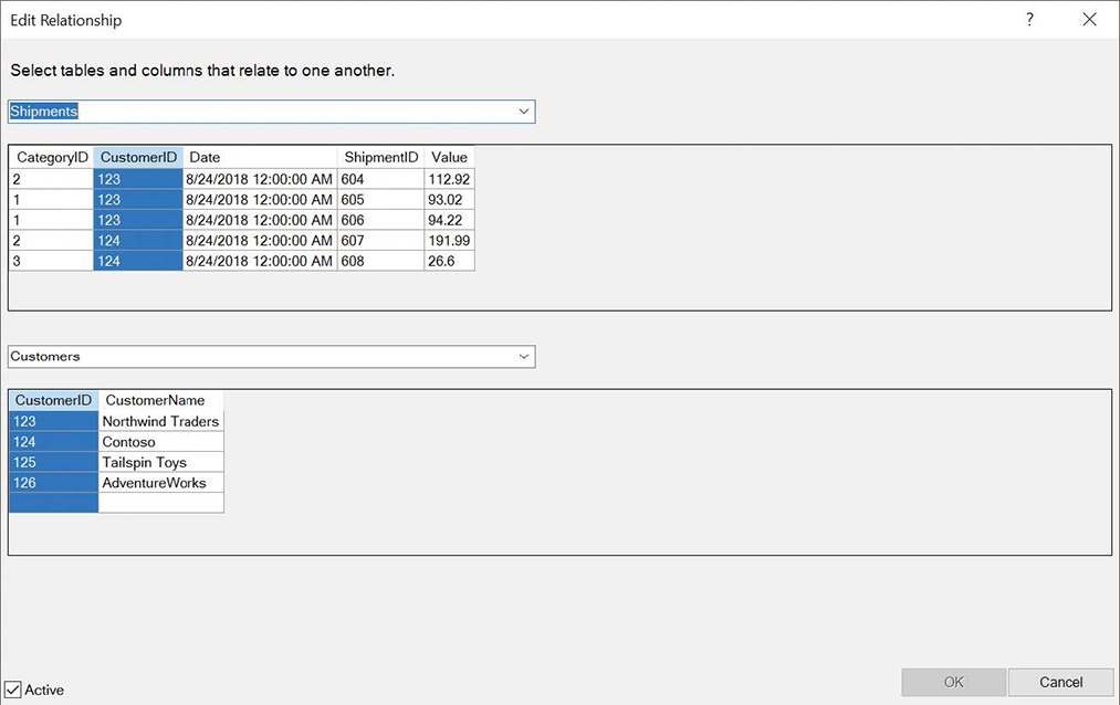
Edit relationships between tables in the Data Model. In the Edit Relationship dialog box, change the tables and fields that form the relationship.
Click OK.
To delete a relationship
In Power Pivot, click Manage Relationships.
In the Manage Relationships dialog box, click the relationship you want to delete.
Click Delete.
In the confirmation dialog box that appears, click OK.
Click Close.
Analyze data by using Power Pivot
When the Excel product team changed the underlying file format of Excel 2007 from XLS to XLSX, they let users store much more data on each worksheet. Rather than limiting each worksheet to 65,536 rows, you can now store up to 1,048,576 rows of data. In 2007, that larger number of rows seemed more than adequate for most Excel users. It still is, but the powerful business intelligence analysis tools built into Excel led users to import large data sets and to find ways to combine data collections that spanned multiple worksheets.
Originally introduced as an add-in for Excel 2010, Power Pivot is a tool you can use to work with any amount of data, as long as the total file size is less than 2 gigabytes (GB) and takes up less than 4 GB of memory. For such large data collections, you’ll usually work with summaries of your data, though you can focus on specific aspects of the data by sorting and filtering.
![]() See Also
See Also
For more information about creating filters, see “Limit data that appears on your screen” in Chapter 5, “Manage worksheet data.”
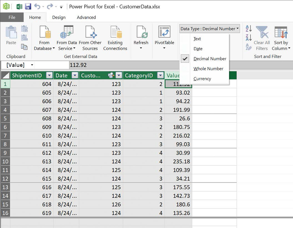
When you bring a data collection into Power Pivot, Excel attempts to identify the data type of each column. The app is usually accurate, but some data types can cause confusion. For example, Excel will occasionally identify currency or accounting data columns as containing regular numbers that include decimal values. If this type of mistake happens, you can always change the column’s data type.
![]() Important
Important
When you change the data type of a column, it might affect the column values’ precision and the results of calculations performed using the data.
Most large data sets contain raw data, such as sales amounts, and rely on the visualization or summary software program to calculate values such as sales tax, commissions, or profit. To add this type of summary to your Power Pivot data, you can define a calculated column. The formula syntax for creating a calculated column is very similar to creating a formula that refers to an Excel table column, so you already have the skills to create them.
As with columns in Excel tables, you can rename and delete Power Pivot columns, but the real analytical power of Power Pivot comes from creating PivotTables from the large Power Pivot data sets. Creating a PivotTable from 10,000 rows of data is useful; creating a PivotTable from 10,000,000 rows can provide incredible insight.
To sort values in a column in ascending or descending order
In Power Pivot, while viewing a table in Data View, click a cell in the column by which you want to sort the table.
On the Home tab, in the Sort and Filter group, do either of the following:
Click Sort Ascending to sort the column’s values in ascending order.
Click Sort Descending to sort the column’s values in descending order.
 Tip
TipThe Sort Ascending and Sort Descending buttons will have different labels depending on the values in the column. For example, a number field will have the label Sort Smallest to Largest, whereas a text field will have the label Sort A to Z.
To clear a sort from a sorted column
In Power Pivot, while viewing a table in Data View, click a cell in the column by which you have sorted the table.
In the Sort and Filter group, click Clear Sort.
To filter values in a column
In Power Pivot, while viewing a table in Data View, click the filter arrow at the right edge of the header for the column by which you want to filter the table.
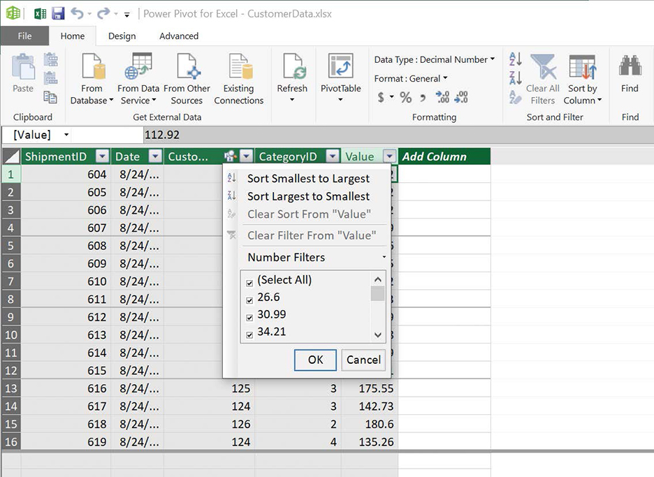
Filter Power Pivot columns by creating rules or selecting specific values. In the filter list, perform either of the following actions:
Click DataType Filters, click the type of filter rule you want to create, create the rule, and click OK.
Select and clear the check boxes to show or hide individual values.
Click OK.
To clear filters applied to a Power Pivot sheet
In Power Pivot, on the Home tab, in the Sort and Filter group, click Clear All Filters.
Or
Click the filter arrow of the column from which you want to remove the filter.
In the filter list, click Clear Filter from “FieldName”.
Click OK.
To change the format of a column
If necessary, in Power Pivot, on the Home tab, in the View group, click Data View.
Click a cell in the column you want to format.
By using the controls in the Formatting group of the Home tab, perform any of the following actions:
Click Data Type, and then click a new data type in the list.
Click Format, and then click a new data format in the list.
Click Apply Currency Format, Apply Percentage Format, or Thousands Separator to apply that format to the column.
Click Increase Decimal or Decrease Decimal to increase or decrease the number of digits shown to the right of the decimal point.
To add a calculated column
In Power Pivot, while viewing a table in Data View, click the top cell in the Add Column column.
Enter = followed by the formula you want to create.
Add fields to the formula by entering [ and then selecting the field that contains the values you want to use in your formula.
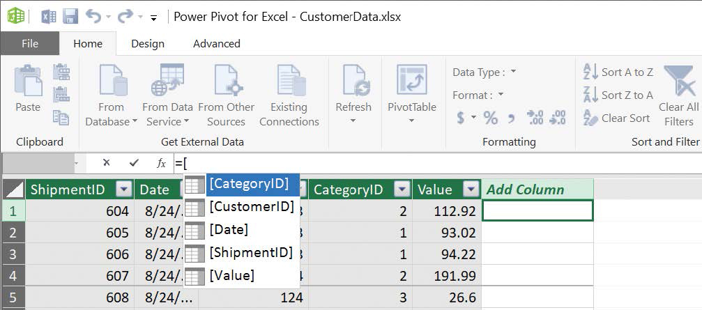
Define a calculated column by using techniques similar to summarizing values in Excel tables. Press Enter.
To rename a column
In Power Pivot, while viewing a table in Data View, double-click the header cell of the column you want to rename.
Enter the new column name.
Press Enter.
To delete a column
In Power Pivot, while viewing a table in Data View, right-click the header cell of the column you want to delete.
Click Delete Columns.
To create a PivotTable from Power Pivot data
In Power Pivot, on the Home tab, click PivotTable.
In the Create PivotTable dialog box, click New Worksheet.
Click OK.
TipExcel creates a PivotTable by using all available data in the Data Model, not just the table that was displayed when you created the PivotTable.
View data by using timelines
Business data often records events at a specific point in time, whether a sale to an individual customer on a specific day or net profit for a quarter or a year. If your data contains a time-based value, such as the day of a sale, you can analyze that data by creating a timeline.
![]() Tip
Tip
Timelines and slicers are built on the same design philosophy: providing a visual indication of the elements included and excluded by a filter. What slicers do for category data, timelines do for chronological data.
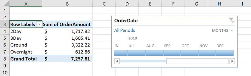
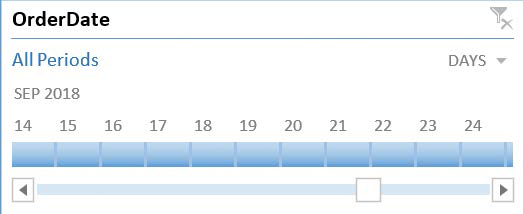
A timeline provides a graphical interface you can use to filter a PivotTable. For table columns that contain individual date values, such as 8/2/2018, the timeline box will recognize those dates and let you filter by year, quarter, month, or day.
You can use the elements within a timeline to select individual increments, such as days or months, or ranges of those same values. As with other objects, such as charts, you can change the appearance of your timeline, resize it, change its appearance, hide or display elements, and delete it when it’s no longer required.
To create a timeline
Click a cell in an Excel table that is based on a connection to an external data source or that is part of the workbook’s Data Model.
On the Insert tab, in the Filters group, click Timeline.
In the Existing Connections dialog box, do either of the following:
Use the tools on the Connections tab to identify the connection you want to filter by using a timeline.
Use the tools on the Data Model tab to identify the Excel table you want to filter by using a timeline.
Click Open.
In the Insert Timelines dialog box, select the check box next to the field by which you want to filter.
Click OK.
To filter a PivotTable by using a timeline
Create a timeline based on an Excel table that has been used to create a PivotTable.
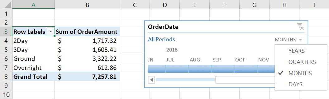
Click Time Level in the upper-right area of the timeline, and then click the time level you want to use (such as months, quarters, or days).
Select the increment by which you want to filter in your timeline. In the scrolling time display, do any of the following:
Click the increment you want to display.
Select multiple increments by holding down the Ctrl key and clicking the increments you want to display.
Select a range of increments by clicking the first increment in the range and then, while holding down the Shift key, clicking the last increment in the range of dates you want to display.
To clear a timeline filter
In the timeline, click the Clear Filter button at the right end of the title bar.
To change the appearance of a timeline
Click the timeline.
On the Options tool tab of the ribbon, in the Timeline Styles gallery, click the style you want to apply.
To resize a timeline
Click the timeline.
Drag any of the handles on the timeline to change its size, as follows:
Drag a handle in the middle of the top or bottom edge to make the timeline shorter or taller.
Drag a handle in the middle of the left or right edge to make the timeline wider or narrower.
Drag a handle in the corner of the timeline to change its shape both horizontally and vertically.
Or
Click the timeline.
On the Options tool tab, in the Size group, do either (or both) of the following:
In the Height box, enter a new height for the timeline, and then press Enter.
In the Width box, enter a new width for the timeline, and then press Enter.
To hide or display timeline elements
Click the timeline.
On the Options tool tab, in the Show group, select or clear any of these check boxes:
Header
Selection Label
Scrollbar
Time Level
To change a timeline caption
Click the timeline.
On the Options tool tab, in the Timeline group, in the Timeline Caption box, enter a new caption for the timeline.
Press Enter.
To delete a timeline
Right-click the timeline, and then click Remove Timeline.
Bring in external data by using Power Query
Excel includes a wide range of analytical tools you can use to generate useful insights from your data. Excel 2019 includes Power Query, a versatile tool you can use to manage external data sources effectively. Unlike in previous versions of Excel, in which you needed to install Power Query as a separate add-in, Power Query is built into Excel 2019.
![]() Tip
Tip
You don’t need to enable the Data Analysis add-ins to use Power Query, but they work best together.
You can create data connections to many different sources:
Files These include Excel workbooks, CSV files, XML files, and text files.
Databases These include Microsoft SQL Server, Access, SQL Server Analysis Services, Oracle, IBM DB2, MySQL, PostgreSQL, Sybase, and Teradata.
Microsoft Azure These include Azure SQL Database, Azure Marketplace, Azure HDInsight, Azure Blob Storage, and Azure Table Storage.
Other sources These include the web, Microsoft SharePoint lists, Hadoop files (HDFS), Facebook, Salesforce, and other sources with available Open Database Connectivity (ODBC) drivers.
Creating a query involves identifying the type of data source to which you want to connect, selecting the software from among that type’s choices, and providing any necessary credentials to access the data source. Some systems require you to log on to an account to access your data, for example.
After you define your data connection, you can specify which elements of the data source you want to import. Many Excel files and databases contain multiple tables, so you can select which of them to bring in.
After your query data appears in an Excel table, you can work with it as you would any other data. You can unlock more powerful tools by turning on the Data Analysis add-ins and adding the Excel table to the Data Model. When the Excel table is part of the Data Model, you can define relationships between it and other tables to enhance your analysis.
Some data sources are poorly designed and don’t include an index field, which contains a unique value for each row. If that’s the case, you can add an index, starting at the value of your choice and increasing in the increment you want, to provide the tool you need to create relationships between tables.
As with other Excel workbook objects, you can edit your queries after you create them. You can select which columns to include in or exclude from your results, change the query’s name, edit or undo a change, and even delete your query to generate the result you want.
To create a query
In the Excel workbook, on the Data tab of the ribbon, in the Get & Transform group, click New Query.
Use the tools on the list to identify the data source to which you want to connect.
In the Import Data dialog box, click the data source you want to query, and then click Open.
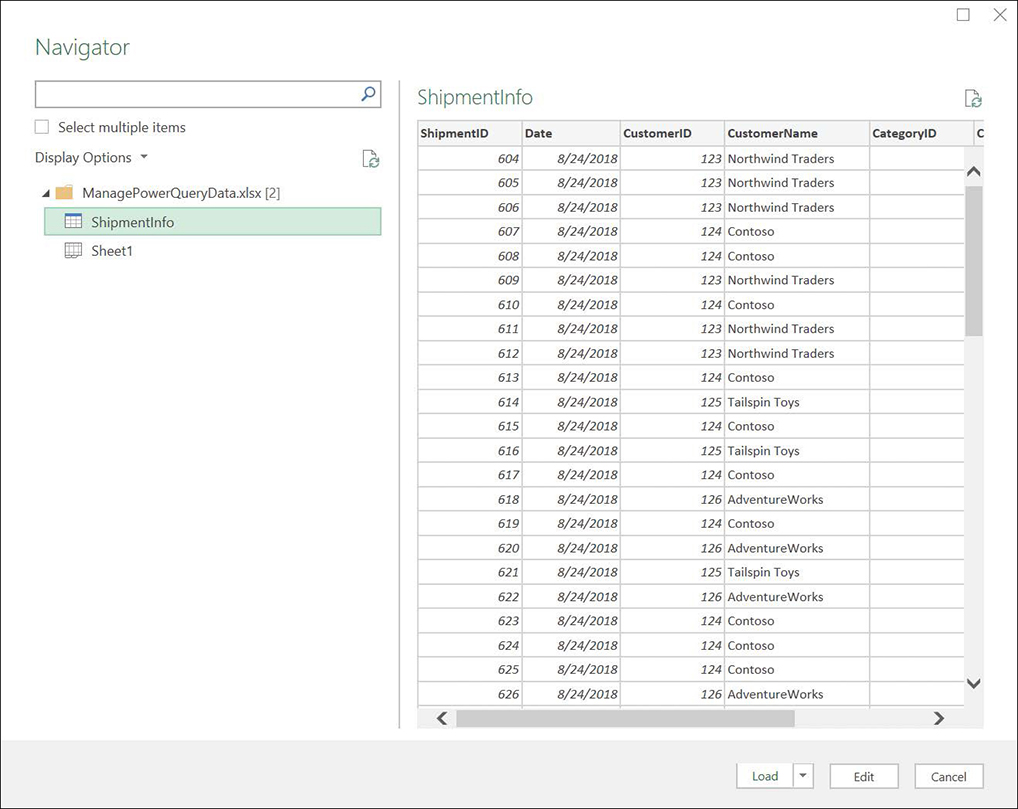
In the Navigator, click the data source you want to query.
Or
Select the Select multiple items check box, and then click the data sources you want to query.
Select the items you want to include in your query.
Click Load.
To add query data to the Data Model
In the Excel workbook, click any cell in the Excel table that contains the query data.
On the Power Pivot tab, in the Tables group, click Add to Data Model.
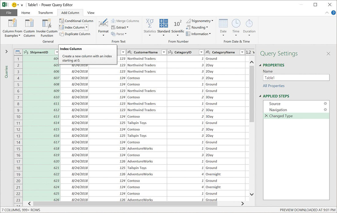
To add an index column to a query
In the Excel workbook, click any cell in the Excel table that contains the query data.
On the Query tool tab of the ribbon, in the Edit group, click Edit.
In the Query Editor, on the Add Column tab of the ribbon, in the General group, click Add Index Column.
Or
Click the Add Index Column arrow (not the button), and then use the tools in the list to define the starting point for your index.
In the Query Editor, on the Home tab of the ribbon, in the Close group, click Close & Load.
To choose columns to include in your query results
In the Excel workbook, click any cell in the Excel table that contains the query data.
On the Query tool tab, click Edit.
In the Query Editor, on the Home tab, in the Manage Columns group, click Choose Columns.
In the Choose Columns task pane, select the check boxes next to the columns you want to keep in your query results.
Click OK.
To remove a column from your query results
Open the query in the Query Editor.
Click a cell in the column you want to remove.
In the Manage Columns group, click Remove Columns.
To change the data type of a column
Open the query in the Query Editor.
Click a cell in the column you want to edit.
On the Home tab, in the Transform group, click Data Type, and then click the new data type for the column.
To change the name of a query
Display the query in the Query Editor.
If necessary, on the View tab of the ribbon, in the Show group, click Query Settings to display the Query Settings task pane.
In the Query Settings task pane, in the Name box, enter a new name for the query.
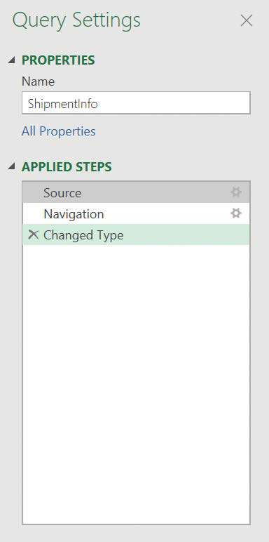
Use the Query Settings task pane to rename and edit queries.
To undo a change to a query
Display the query in the Query Editor.
If necessary, click Query Settings to display the Query Settings task pane.
In the Applied Steps list, point to the change you want to delete, and then click the delete icon that appears to the left of the change.
If necessary, in the Delete Step confirmation dialog box, click Delete to finish deleting the change.
To edit a change to a query
Display the query in the Query Editor.
If necessary, click Query Settings to display the Query Settings task pane.
In the Applied Steps list, point to the change you want to edit, and then click the action icon (it looks like a gear or cog) that appears to the right of the change.
In the dialog box that appears, edit the properties of the change.
Click OK.
To close a query and return to Excel
In the Query Editor, on the Home tab, in the Close group, click Close & Load.
If necessary, in the dialog box that appears, click Keep to keep your changes.
To delete a query
In the Excel workbook, click any cell in the Excel table that contains the query data.
On the Query tool tab, in the Edit group, click Delete.
In the Delete Query dialog box that appears, click Delete.
Skills review
In this chapter, you learned how to:
Define a Data Model
Define relationships between tables
Analyze data by using Power Pivot
View data by using timelines
Bring in external data by using Power Query
Practice tasks

The practice files for these tasks are located in the Excel2019SBSCh15 folder. You can save the results of the tasks in the same folder.
Define a Data Model
Open the DefineModel workbook in Excel, and then perform the following tasks:
Open the Excel Options dialog box.
Enable the Data Analysis add-ins.
Close the Excel Options dialog box.
Add the Customers and Shipments tables to the Data Model.
Define relationships between tables
Open the DefineRelationships workbook in Excel, and then perform the following tasks:
If necessary, add the two Excel tables in the workbook to the Data Model.
Display the Data Model in Diagram View.
Create relationships between the following pairs of tables:
Customers and Shipments based on CustomerID
Categories and Shipments based on CategoryID
Close the Data Model and return to the main workbook.
Analyze data by using Power Pivot
Open the AnalyzePowerPivotData workbook in Excel, and then perform the following tasks:
Display the Data Model in Data View.
On the Home tab of the ribbon, click PivotTable.
Create a PivotTable that displays the customers’ names as the row headers and the total value of their shipments in the Values area.
Change the data type of the Value field to Currency.
Add a calculated column that adds a 3-percent surcharge to each shipment to account for increased fuel costs.
View data by using timelines
Open the ViewUsingTimelines workbook in Excel, and then perform the following tasks:
Click any cell in the PivotTable in the Summary worksheet.
Create a timeline that lets you filter the PivotTable by using the values in the OrderDate field.
Using the timeline, filter the PivotTable to display the Sum of OrderAmount for November 2018, then for November and December 2018, and for the third quarter of the year.
Change the timeline’s appearance so it has a yellow and black theme.
Clear the filter, and then delete the timeline.
Bring in external data by using Power Query
Open the CreateQuery workbook in Excel, and then perform the following tasks:
Using the tools on the Data tab of the ribbon, use Power Query to import the table named ShipmentInfo from the ManagePowerQueryData workbook.
Add the query’s results to the Data Model.
Remove the CustomerID and CategoryID fields from the query’s results.
Change the name of the query.
Save your work and return to the main Excel workbook.