
Chapter at a glance
Adjust
Adjust the width of columns to fit your data, Changing column widths
AutoFill
Quickly create a series of numbers or numbered text, Extending a series with AutoFill
Name
Name cells and ranges for easy reference, Selecting and naming cell ranges
Copy
Copy a cell or range in an operation, Copying one or more cells to many
IN THIS CHAPTER, YOU WILL LEARN HOW TO
Modify Excel options.
Format as you enter text.
Extend a numeric series.
Extend a series based on adjacent data.
Assign names to cells and ranges.
Select and navigate by using the keyboard.
Customize and move column widths and row heights.
This chapter will cover some of the basics of spreadsheet construction and maintenance, including techniques for entering and organizing data and ways to manipulate cells and move among them.
If you are familiar with Microsoft Excel 2010, you will notice very little functional difference at first glance on the Home tab, beyond the new simplified Microsoft Office look. However, if you are logged into a Windows Live, Microsoft SkyDrive, Outlook, or Hotmail account, your name and image may appear among the window controls in the upper-right corner of the Login menu, This allows you to access your account settings, switch accounts, and even change your profile photo. One more small difference is that the Full Screen button (formerly on the View tab) now lives in the upper-right corner along with the window controls. These changes were designed to facilitate performance on a range of devices and displays, from phones to desktops, tablets, and TVs.
See Also
For more information, see Chapter 4.
So, it may look like not much has changed—Excel is a “mature” application, after all—but there are some great new features, hidden in buttons and commands, some of which may just happen before you know they’re there. Exploring the other tabs on the ribbon will reveal more, especially on the Insert and Data tabs.
In this chapter, you’ll learn some of the most useful basic techniques for creating and organizing worksheets and workbooks, entering data, making calculations, analyzing data, and preparing for presentation. In such a short discussion, we won’t be able to tell you everything there is to know about Excel, but we encourage you to explore at every juncture. When a dialog box is open for a procedure, examine its contents; click other tabs; try a procedure in a different way; use your own data after trying the practice files, and so on. Remember, you can undo up to 100 actions, with a few exceptions like saving workbooks and deleting worksheets.
Practice Files
To complete the exercises in this chapter, you need the practice files contained in the Chapter18 practice file folder. For more information, see Download the practice files in this book’s Introduction.
The general rule of thumb is to put whatever you have the most of into rows, and try to fit all of your columns across a sheet of paper, even if it will print in landscape mode. That way, if you have more than one page of data, the bottom of a page leads naturally to the top of the next page, not the top of the next column. Your audience is more accustomed to “paging down” than “paging right.”

Think about the audience and the output you plan to produce. Size matters: are you printing, emailing, or web-publishing your work? Content matters: will you share your work, or is it just for your own use? Details matter: do you need an executive summary? Appearance matters: how about presentation graphics? Documentation matters: do you need to make sure others know how to use your workbooks in the future without your personal intervention? Sometimes, it’s all (or most) of the above.
Generally, the more people you plan to share with, the less data you should share. Find ways to summarize—this is what analysis is all about. It’s almost impossible to comprehend the big picture when you’re looking at details. Sending the VP a raw worksheet with thousands of rows of data probably won’t get your point across as well as a summary table with a few rows and columns and an accompanying chart.
Luckily, you can start small and then create whatever you need later. Virtually everything else in the Excel portion of this book will help you to craft your data to address the questions posed earlier.
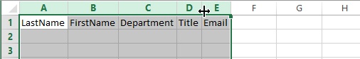
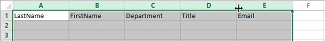
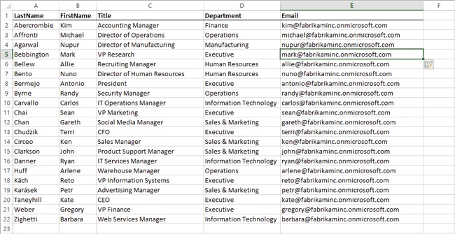
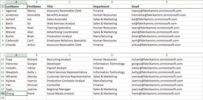
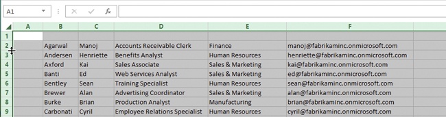
One fundamental requirement of any Excel user is to make sure all your data is visible and readable. If it is not, column widths are probably part, if not all, of the problem. The default 64-pixel column width was chosen to accommodate a typical formatted numeric entry such as $1,234.56 without adjustment. When you enter numbers, Excel usually adjusts the width of the column to accommodate the entry. Not so with text, however. The following graphic shows a simple example of what is possibly the most common spreadsheet task of all time—a list.
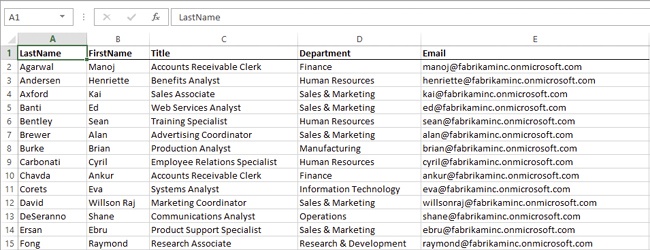
A simple list can be used for various purposes; for example, for generating mailing lists, organization charts, and departmental rosters. Most times, it is best to keep your detail data simple and easy to edit and manipulate. Then you can create additional sheets to summarize or otherwise interpret the data.
In this exercise, you begin creating a sheet like this to illustrate a few techniques.
Set Up
You don’t need any practice files to complete this exercise. Start Excel and follow the steps.
Click the File tab and click New to display the opening screen, if it is not already visible.
Click Blank Workbook to create a new file with a clean, new worksheet.
Enter LastName in cell A1 (don’t press Enter), then press the Tab key to activate the next cell to the right.
Enter FirstName in cell B1, then press the Tab key.
Enter Department in cell C1, then press the Tab key.
Enter Title in cell D1, then press the Tab key.
Press the Home key to select cell A1.
Press and hold the Shift and Ctrl keys and then press the Right Arrow key to select all the headings you just entered. Notice that all the columns are the same default width.
In the Font group on the ribbon, click both the Bold button and the Bottom Border button. If the Bottom Border button is not currently visible, click the arrow next to the Border button and select Bottom Border from the list.
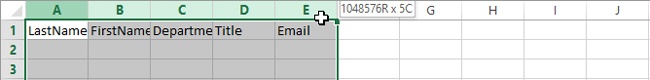
Click the column heading letter A to select the entire column, then, still holding the mouse button down, drag through the column letters from A to E. Notice as you drag that Excel displays a ScreenTip showing the dimensions of the selected range, which in this case is 1,048,576 rows deep (all the rows in the worksheet, because you selected the entire column) by 5 columns wide. Excel designates rows by appending an R to the row number, and it does the same for columns, with a C to the column number, as shown in the ScreenTip.
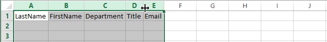
Point to the border line to the right of any selected column letter until it becomes a double-headed arrow pointer, and then double-click to auto-fit all selected columns to their widest entries. Notice that the columns are now different widths.
With the columns still selected, click the right border line of any selected column heading (don’t double-click) and drag it to the right to make it wider. Notice that not only are all of the selected columns wider now, they are also all the same width.

The great thing about this feature is that you don’t have to scroll down a long worksheet to determine if a column is wide enough for everything it contains; simply double-clicking the column-letter border essentially does that for you. If a column seems too wide after auto-fitting, it may point out a problem somewhere else, such as data entered or imported incorrectly into a cell, or a label out of place.
Tip
It works for rows, too. Excel increases row height automatically if you increase the font size or apply the Wrap Text format, but does not decrease it automatically if the cell contents no longer warrant it. Just like columns, you can drag to resize rows, or you can auto-fit them by double-clicking the border below the row number to fit its tallest entry.
A worksheet can be a façade; what is displayed isn’t necessarily all there is to it. The displayed values on the screen may not be exactly the same as the underlying values that appear if you select a cell and look in the formula bar. How numeric entries are formatted makes a huge difference in how they appear.
To Excel, everything is a value, including text. What you enter and how you enter it changes the way that Excel responds to the entry. Fractions, dates, times, currency, scientific values, and percentages are all just raw numeric values that are formatted so that they are displayed in familiar ways. This allows Excel to perform calculations on the raw numbers, while allowing you to view the more easily readable formatted values.
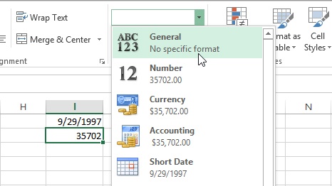
For example, Excel uses numeric values to calculate dates. The serial (sequential) value representing Christmas Day 2013 is 41633, which is the actual number of days that have elapsed since (and including) January 1, 1900. If a cell containing this number has the Short Date format applied, it appears in the more understandable form 12/25/2013.
Tip
Enter any date into a cell, then click the Number Format drop-down menu (located in the Number group on the Home tab), and click General to format the date so that it displays its serial value. Then you can click one of the Date formats to display the number as a date again.
Important
Applying a Date or Time format to a number appears to actually change the underlying value in the formula bar, but you can always change it back by simply applying a numeric format.
In this exercise, you’ll find that although you can always apply formatting by using buttons on the ribbon, when entering numeric values, you can specify many kinds of formats “by example” as you enter data, including currency, percentages, and dates.
Set Up
You don’t need any practice files to complete this exercise. Start Excel, open a blank workbook, and follow the steps.
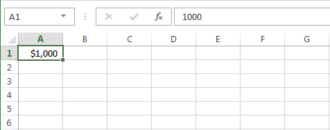
In cell A1, enter $1000 and press Enter.
Press the Up Arrow key to reselect the cell, and notice the difference between the entry in the cell itself and the entry as shown in the formula bar above.
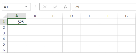
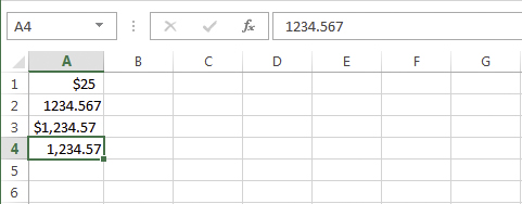
Now, in cell A1, enter 25 (no dollar sign) and notice that even though you replaced the number you first entered in dollars, the cell still displays a dollar sign, because the cell is formatted as currency. After you format a cell “by example,” it stays in that format until you explicitly change it by using formatting commands.
In cell A2, enter 1234.567 and press Enter, then enter $1234.567 and press Enter, then enter 1,234.567 and press Enter (making sure to add the comma). If you select each cell that contains the numbers you just entered, you’ll notice that the numbers all look exactly the same in the formula bar.
This example illustrates the difference between the formatted values displayed on the worksheet and the underlying values displayed in the formula bar. It also shows that Excel interprets numeric entries based on the way you enter them and applies formatting accordingly. Entering a dollar sign in front of a number tells Excel to format the entry as currency, which Excel dutifully applies for you. This particular currency format (there are several) includes a dollar sign and comma separators, and rounds the decimal portion to two places. Because you entered a comma separator along with the value in cell A4, Excel applied a different currency format without dollar signs. However, as shown in the formula bar, the formatting only appears on the worksheet. The actual values you enter are not altered. The underlying values in cells A2, A3, and A4 are identical; only the formatting is different.
Excel provides a few tools you can use to quickly fill a cell range with a series of numbers, dates, formulas, or even text ending with serial numeric values such as Q1, Q2, and so on. For example, you could enter three numbers or dates into adjacent cells, select them, and then drag to extend a series based on the selected cells. They need not be consecutive. Excel extrapolates the numeric or date series by using the example increments.
In this exercise, you’ll create simple series by dragging or by using commands on the ribbon.
Set Up
You don’t need any practice files to complete this exercise. Start Excel, open a blank workbook, and follow the steps.
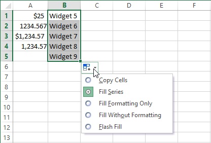
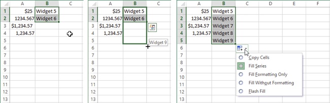
In cell B1, enter Widget 5.
In cell B2, enter Widget 6.
Click cell B1 and drag to cell B2 to select both cells.
Click the tiny black dot at the lower-right corner of the selection, called the selection handle, and drag down to cell B5.
Excel displays a ScreenTip (Widget 9) showing you what the value in that cell will be.
Release the mouse button to apply the fill and reveal a numbered series of widgets.
Click the AutoFill Options menu—the little box that appears near the lower-right corner of the selection after dragging—to display a few additional options you can apply even after you’re done. The default option selected is Fill Series, which is what you want, so you can press Esc to dismiss the menu.
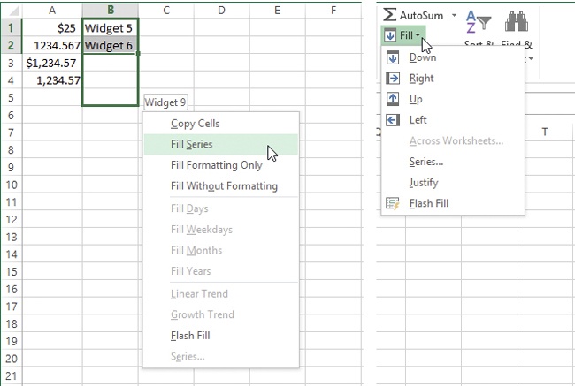
AutoFill makes it easy to extend a series of numbers, dates, or text/numeric entries, as in the Widgets example. You can also click and drag the fill handle by using the right mouse button. Then, instead of immediately extending the series, Excel presents you with a menu of options first, including trends and dates. (Commands appear gray if they are not applicable to the selected values.) You can also use the Fill menu, located in the Editing group on the Home tab, to apply different types of fills.
See Also
For more about using AutoFill with formulas, see Chapter 19. For more about filling across worksheets, see Creating a multisheet workbook in Chapter 22.
Another helpful feature of AutoFill is that it recognizes certain text/number combinations as special cases. For example, if you enter Q1 into a cell, and then drag the fill handle, you’ll notice that Excel extends it, stops at Q4, and keeps repeating Q1, Q2, Q3, and Q4, over and over, rather than copying the cell or extending the numeric series. Excel recognizes that these are common designations used to specify annual quarters, and will perform the same trick if you start with “Quarter 1” or “1st Quarter.”
Tip
If you really just want to make copies, you can temporarily suppress AutoFill by holding down Ctrl while dragging the fill handle.
The new Flash Fill command in the Data Tools group on the Data tab is a clever cousin of AutoFill. It evaluates example data, compares it to existing data in adjacent cells, tries to determine a pattern, and suggests entries for you. (The Flash Fill command is also available on the Fill menu that appears when you click the Fill button in the Editing group on the Home tab.)
For example, suppose your company switches to a brand new email domain, and you need to create a new set of unique email addresses for all of your employees.
In this exercise, you’ll quickly create a list of email addresses and combine first and last names from separate cells into a single cell.
Set Up
You need the Fabrikam-Management_start.xlsx workbook located in the Chapter18 practice file folder to complete this exercise. Open the Fabrikam-Management_start.xlsx workbook, and save it as Fabrikam-Management.xlsx.
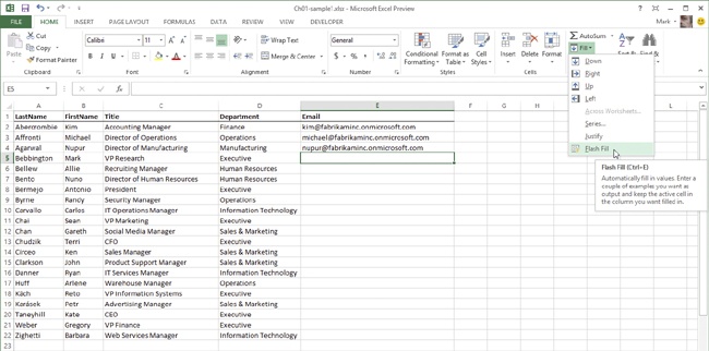
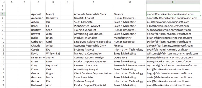
Open the Fabrikam-Management.xlsx sample workbook and make sure cell E5 is selected.
Click the Fill menu in the Editing group on the Home tab, and click Flash Fill.
These email addresses simply use employees’ first names with a common email domain. Excel correctly determined the desired outcome, even though those first names were several columns away. (Both columns need to be part of the same table, though.) Excel analyzed the examples entered into cells E2 through E4, and then with the next cell in the table selected, Flash Fill finished the entries and stopped at the end of the table, saving a lot of time entering text. Flash Fill doesn’t always get it right, but if not, add more examples.
Tip
When you enter a complete email or web address into a cell, Excel formats it as a hyperlink (blue underlined text). When you click a hyperlink, it opens the target; for example, an email program, web browser, or file. Excel actually applies the hyperlink format as a second action after you press Enter. If you would rather not have active hyperlinks in your worksheet (as in this example), press Ctrl+Z immediately after you enter to undo the last action. Because there were actually two actions that took place after you pressed Enter, (you entering the value in the cell, and Excel applying the hyperlink), only the hyperlink is undone, and the unlinked text remains.
One of the most common list-management tasks is managing contact or address lists. For example, first and last names are often kept together in the same cell (or the same record in an imported database). But sometimes first and last names are kept separate; at times you need just the first or last name. Flash Fill offers options for combining (concatenating) or splitting (parsing) cell entries.
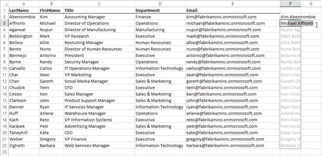
Select cell F2 and enter Kim Abercrombie.
In cell F3, begin entering Michael Affronti. Even before you finish entering the word Michael, Excel fills in the rest of the name in cell F3, and simultaneously shows what Flash Fill thinks you’re trying to do in the cells following.
Press Enter to accept the Flash Fill suggestions.
Double-click the right border of column heading F to auto-fit its contents.
Select cell G2 and enter Kim in Finance.
Select cell G3 and enter Michael in Operations.
Select cell G4 and begin entering Nupur in Manufacturing.
Press Enter to accept the suggested entries.
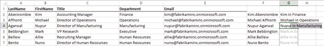
This time, it took three examples before Flash Fill figured out the pattern, including an incorrect guess on the second entry. Just keep entering text if the suggestions don’t work.
Similarly, you could use Flash Fill to split, or parse, the full names you entered in column F back into individual cells by simply entering Abercrombie into cell H2, and Affronti into cell H3. Flash Fill springs to life, offering correct suggestions by around the third letter of the second name. This is one very powerful feature that you’ll want to experiment with.
You know how to select a cell—just click it. You know how to select multiple cells—just click and drag to select a range. In Excel, you can also select multiple nonadjacent (also known as noncontiguous) ranges, a technique that comes in handy if you need to apply formatting, styles, or certain editing techniques to noncontiguous cells. You can apply most kinds of formatting to noncontiguous ranges, but many editing techniques are prohibited, including copying and pasting.
Sometimes, especially in large worksheets, it is helpful to assign names to cells and ranges. A name is simply an easy way to identify specific cells. Names can be used to quickly select ranges, or they can be used in formulas as proxies for cryptic cell addresses or to identify the results of other formulas; for example, net_profit. Names can also be used to identify cells containing often-used static values such as sales_tax_rate. Names can be easier to remember and work with than cell or range addresses.
In this exercise, you’ll select nonadajacent cells and assign names to cells.
Set Up
You need the Fabrikam-Management2_start.xlsx workbook located in the Chapter18 practice file folder to complete this exercise. Open the Fabrikam-Management2_start.xlsx workbook and save it as Fabrikam-Management2.xlsx.
Open the Fabrikam-Management2.xlsx workbook.
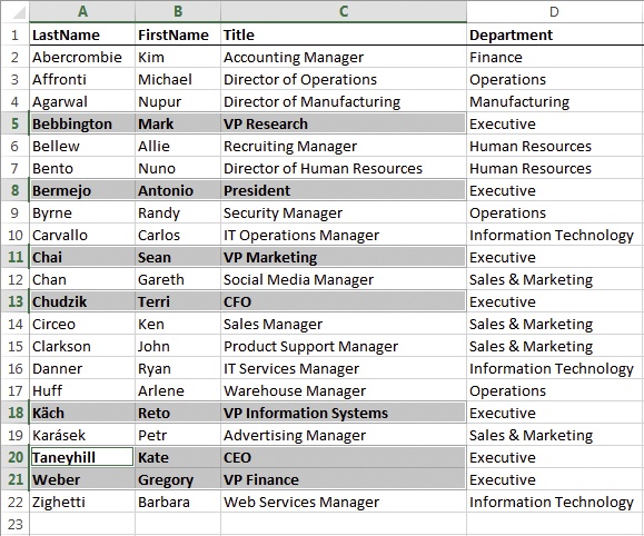
Click cell A5 and drag to the right, selecting cells A5:C5.
Note that this is how Excel identifies a cell range; the ID of the cell in the upper-left corner and the ID of the cell in the lower-right corner, separated by a colon.
Hold the Ctrl key while selecting the corresponding cells in columns A through C for each of the other members of the Executive department (the 1x3 cell ranges A8:C8, A11:C11, A13:C13, A18:C18, and a 2x3 range, A20:C21).
While still holding the Ctrl key, press the B key to apply Bold formatting to all the selected cells. Alternatively, you could click the Bold button on the Home tab of the ribbon.
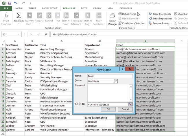
Select all the email addresses.
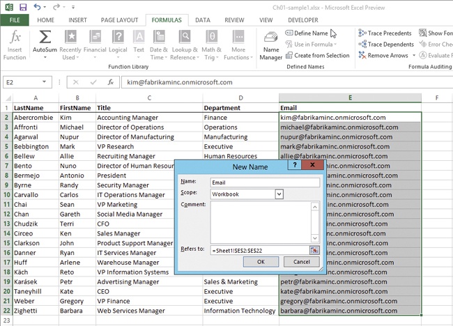
Click the Formulas tab on the ribbon.
Click the Define Name command in the Defined Names section to display the Define Name dialog box.
The first email address is displayed and highlighted in the Name field of the dialog box.
Enter Email. This replaces the highlighted email address.
Press Enter and then look at the box on the left side of the formula bar; this is called the Name box, and it normally displays the address of the active cell, unless a named cell or complete named range is selected. After you click Enter, the Name box should display the name Email.
Click to select any cell outside the Email range.
Click the arrow next to the Name box and click Email, which reselects the named range. You can also click the Name box and enter email (case-insensitive) to select the associated cell or cells.
See Also
For more information, see Chapter 19.

Tip
When you first create a defined name, you can use the Scope options in the New Name dialog box to limit the usage of the name to a specific sheet in the workbook (which, of course, doesn’t matter if there is only one sheet). Normally, Workbook is the selected Scope, meaning that you can use the name on any sheet. If you specify a sheet in the Scope drop-down list, you will only be able to use the name on that sheet.
You can define multiple names at once by using the Create From Selection command on the Formulas tab of the ribbon. Remember that when you defined the name Email in the previous example, you selected the data but not the column heading. When you use the Create From Selection command, you need to select the headers along with the data.
In this exercise, you’ll create names by using column headings, and you’ll begin by using a keyboard-selection trick to select the table.
Set Up
You need the Fabrikam-Management3_start.xlsx workbook located in the Chapter18 practice file folder to complete this exercise. Open the Fabrikam-Management3_start.xlsx workbook and save it as Fabrikam-Management3.xlsx.
Open the Fabrikam-Management3.xlsx workbook.
Click cell A1 to select it.
Hold down the Shift and Ctrl keys and then press the Right Arrow key to select the top row of the table.
While still holding Shift and Ctrl, click the Down Arrow key to select the entire table.
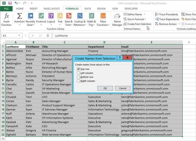
Click the Formulas tab if it is not already active, and click the Create From Selection command in the Defined Names group.
Click the Left Column option in the Create Names From Selection dialog box to deselect it, because you want to create names just from the column headers at this time.
Click OK to create a set of names based on the column headers you selected.
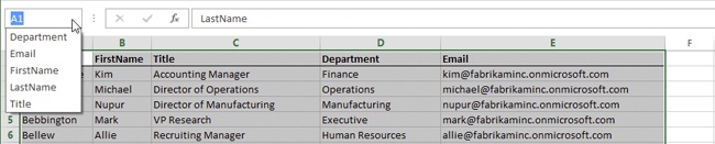
Click the Name box in the formula bar to display the list of names you just created.
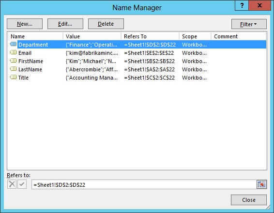
Click the Name Manager command on the Formulas tab of the ribbon for another way to view the names you just created, including the ranges (shown in the Refers To column) and values associated with the names.
See Also
For more information, see Chapter 19.
In the previous exercise, you used a keyboard-navigation technique to select a table. Although using the pointer for selecting and navigating is okay, using keyboard shortcuts can save time, frustration, and repetitive movements, especially when working with larger worksheets.
In this exercise, you’ll navigate between and among regions, which are defined as blocks of contiguous cells.
Set Up
You need the Fabrikam-Employees_start.xlsx workbook located in the Chapter18 practice file folder to complete this exercise. Open the Fabrikam-Employees_start.xlsx workbook, and save it as Fabrikam-Employees.xlsx.
Open the Fabrikam-Employees.xlsx workbook. Make sure that cell A1 is selected.
Hold down Ctrl and press the Down Arrow key to jump to the last entry in column A.
While pressing Ctrl, press the Down Arrow key again and notice that cell A1048576 is selected—the last row in the worksheet.
While pressing Ctrl, press the Up Arrow key to return to the previous location (cell A68).
While pressing Ctrl, press the Right Arrow key to jump to the last active cell in the table (cell E68).
While pressing Ctrl, press the Up Arrow key to jump to the top of the table (cell E1).
While pressing Ctrl, press the Left Arrow key to jump back to cell A1.
Click the Sheet 2 tab at the bottom of the workbook.
Make sure that cell A3 is selected, then hold down Ctrl and press the Right Arrow key, pause, then repeat this three more times, pausing to notice what happens each time. Cell H3 should be selected.
Now hold down Ctrl and Shift together, and press the Down Arrow key to select the data in column H.
Holding Ctrl and Shift, press the Left Arrow key to select the region F3:H21.

When you press any Ctrl+Arrow combination when an empty cell is selected, the selection moves to the first active cell in the next region. If you do this when an active cell is selected, the selection moves to the last active cell in the same region. If there are no active cells in the direction you move, Excel selects the last available cell on the worksheet.
You probably, already know plenty about clicking and dragging; these are core competencies of anyone who uses a computer. Things work differently in Excel than in writing apps, considering the grid or “graph paper” model. Word-processing programs are linear; most text-based documents are essentially one long string of characters. Excel is modular; you can put strings of characters into each cell, like tiny books on a million-shelf bookcase (1,048,576, to be exact). Of course, the tiny books have skills. For now, let’s drag stuff around.
See Also
For more information about formulas and functions, see Chapter 19.
In this exercise, you’ll select and drag cell regions to new locations on a worksheet, and you’ll quickly adjust column widths and row heights afterward.
Set Up
You need the Fabrikam-Employees.xlsx workbook created in the previous exercise to complete this exercise. Or open the Fabrikam-Employees.xlsx workbook located in the Chapter18 practice file folder and save it as Fabrikam-Employees.xlsx.
Open the Fabrikam-Employees.xlsx workbook.
Click the Sheet2 tab at the bottom of the workbook window.
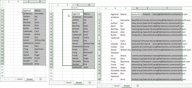
Select the region C3:D21.
Point to one of the borders of the selection, until a 4-headed arrow pointer appears.
Click and drag the region one cell up and one cell to the left (cell B2 becomes the upper-left corner).
Select the region F3:H21, then drag it one cell up and two cells to the left (adjacent to the first region).
Notice that in some of the cells, single letters are wrapping within the cells, other entries are cut off, and others extend beyond the cell borders.
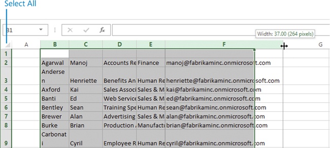
Click the border to the right of column F and drag the column header to the right to make all selected columns wider.
All the entries fit in the cells now, but some columns are too wide and some rows are too deep, so click the Select All button located at the intersection of the row and column headers to select all the rows and columns in the worksheet.
Double-click any border between column headers to auto-fit all columns to their widest entries.
Double-click any border between row headers to auto-fit all rows to their tallest entries (notice that the double-headed arrow pointer points up and down when manipulating row heights).
In this example, there was an intentionally introduced “issue” to illustrate one of the problems that may crop up when moving cells around. The cells containing first names were needlessly formatted with text wrapping turned on (it happens), which is why even individual letters wrapped within cells (for example, see cell B3 in the “before” graphic). Excel makes the row taller when text wraps in a cell, but it does not readjust the row height if you widen the column enough to avoid wrapping. To fix this, we first made the cells too wide, then we auto-fit both the rows and the columns.
If you want, you can turn off text wrapping.
Select the column containing the first names (column B in the “after” graphic earlier).
Click the Wrap Text button twice (the button is located in the Alignment group on the Home tab): once to turn wrapping on in all the selected cells, and once to turn it off.
The Wrap Text button should turn gray when text wrapping is on, and it turns white again when turned off.
Often you just need to move things around in your workbooks, and in a grid like Excel, simple copying and pasting is a needlessly awkward way of doing it. If your worksheet is set up properly, you should be able to drag entire rows and columns around without too much trouble. You simply select and drag to move and replace, or hold down Ctrl and drag to move and insert.
In this exercise, you’ll move rows and columns and copy them, too.
Set Up
You need the Fabrikam-Employees.xlsx workbook created in the previous exercise to complete this exercise. Or open the Fabrikam-Employees.xlsx workbook located in the Chapter18 practice file folder and save it as Fabrikam-Employees.xlsx.
Open the Fabrikam-Employees.xlsx workbook, and make sure Sheet1 is selected.
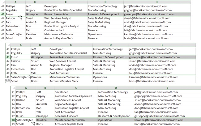
Scroll down to row 43 and click the row header to select the entire row.
Notice that Giuseppe Russo is out of alphabetical order in this table. We’ll fix that.
Point to any part of the selection border around row 43 until the pointer becomes a 4-headed arrow.
Press the Shift key, then click and drag row 43 down.
Notice that while you are dragging, an “I-beam” type insertion cursor appears between rows, indicating the new location.
Release the mouse button when the insertion cursor is between rows 47 and 48.
Tip
If you press Ctrl while dragging a selection, Excel makes a copy of the selected cells and pastes them in the new location rather than inserting them (and replaces the contents of the destination cells). Pressing Ctrl+Shift while dragging both makes a copy of the selected cells and inserts them at the new location.
You use the same techniques when moving and copying columns, too.
In this exercise, you’ll use a handy trick for making a lot of duplicate entries, rather than extending a series of entries.
Set Up
You don’t need any practice files to complete this exercise. Open a blank workbook and follow the steps.
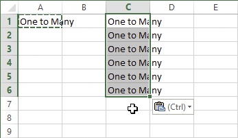
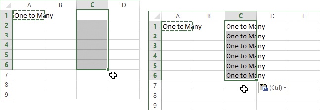
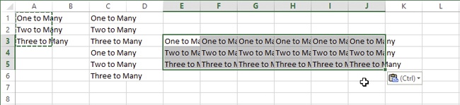
In cell A1, enter One to Many.
Select cell A1 and press Ctrl+C to copy it.
Click cell C1 and drag to select cells C1:C6.
Press Ctrl+V to paste, and notice that Excel fills in the entire range of selected cells with the same entry.
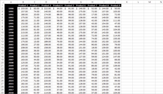
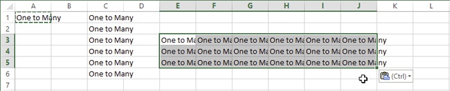
Select cells E3:J5 by dragging through the range, and click Ctrl+V again to paste the entry into a 2-dimensional range.
Select cell A2 and enter Two to Many.
Select cell A3 and enter Three to Many.
Select cells A1:A3 and press Ctrl+C to copy.
Select cells C1:C6 again and press Ctrl+V to paste.
Select cells E3:J5 again and press Ctrl+V to paste.
Excel repeats the sequence to fill your selections. You can select as many cells as you like before you paste, and Excel will keep repeating the sequence you copied until the range is filled.
Number formatting changes the appearance of numbers, but not the underlying values.
You can apply number formatting as you enter data by using currency symbols, percentage symbols, or commas, or by entering dates “in format.”
You can extend a series of numbers, dates, and even text entries with numeric values by dragging.
Flash Fill learns by example to fill a range of cells based on entries in an adjacent column.
You can assign names to cells to make it easier to remember values, to quickly select ranges, or to create more understandable formulas.
Manipulate borders between column letters to change column widths: double-click to auto-fit all selected columns; drag to make all selected columns the same width.
You can use the Select All button to select the entire worksheet, which is useful for formatting and adjusting row heights and column widths.
Use the Ctrl key with an arrow key to navigate around in a worksheet.
You can drag cells, ranges, or entire rows and columns to move them around. Pressing Shift while dragging allows you to insert the item into the new location. Pressing Ctrl makes a copy in the new location.
In calculations, Excel always uses the underlying values displayed in the formula bar, even though the formatted values displayed on the worksheet may be different.
If you paste a copied cell or range into a larger selected range, Excel repeats the copied cells as many times as necessary to fill the destination range.